Week 11 Network Dynamics and Temporality
It’s About Time!
So far in this class we’ve been mostly working with static networks or snapshots of dynamic networks. That’s enough for most of our needs.
However, many social networks are dynamic in nature. One important use of SNA is to understand how a network would function – and evolve – given its current structure. Such a question is genuinely about network dynamics.
In Week 11, we will:
- Explore ways to conceptual temporality in SNA
- Learn how to construct temporal networks
- Learn approaches to visualizing and analyzing temporal networks
- Explore potential applications of temporal SNA to our projects
Note: You may see people using different words temporal, dynamic, longitudinal interchangeably to describe social networks.
11.1 Getting started with network dynamics
Why temporality in networks matters?
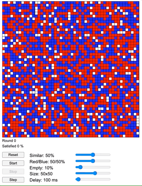
Watch a video below (also link here) about the Schelling’s (1969) Segregation Model to understand the importance of understanding network dynamics.
To further explore the Schelling’s Segregation Model:
- Open http://nifty.stanford.edu/2014/mccown-schelling-model-segregation/
- Adjust Similarity threshold to 50% –> Record rounds
- Adjust Similarity threshold to 75% –> Record rounds
How is the model related to network dynamics?
Approaches to considering time in networks
Temporal information is reflected in networks in several ways:
- Timestamp of an event (when)
- Duration of an event (how long)
- Frequency of of events (how often)
- Time-order / contingency of events (in which temporal order)
There are multiple ways to consider temporal information in network analysis:
1. Time‐aggregated networks
Consider email correspondences among members of an organization. Each week, members of the organization send each other emails. Each email has a timestamp and is directed from one member to one or several members. To generate time‐aggregated networks, one subsets the full record of email exchanges at different start and stop time points and retain any interactions that begin or stop within the window. One straightforward example is to create aggregate email interactions by week and create weekly aggregated networks. By doing so, one can then compare time-aggregated networks across weeks.
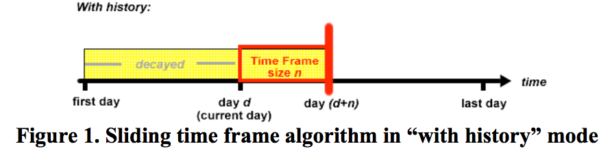
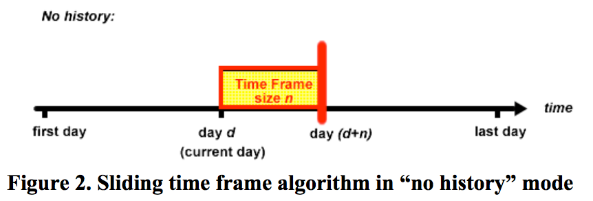
A slightly more complex example of time-aggregated networks is to apply a sliding window on the dataset. To get a sense of how it works, click on the ‘Play’ button of the interactive visualization below. The slider/window will begin to slide rightward, while the window size remains constant. Each snappost you see is a time-aggregated network within its corresponding window.
The sliding window approach can be further enriched. According to Gloor et al. (2004), instead of strictly restricting to events within a time window, you can choose to incorporate information about previous events to each time window. This technique is akin to adding a memory to the time-aggregated networks.
2. Time‐ordered networks
According to Blonder et al. (2012), “Time‐ordered networks represent data observed for a set of interactions that occur at certain times, thereby retaining complete information on the ordering, duration and timing of events.”
This approach retains more detailed temporal information and can be used to answer various questions about flow dynamics. You will have a chance to read more in Blonder et al. (2012) this week (see below).
3. SNA measures with ‘a temporal flavor’
SNA concepts and measures we have explored so far can be extended to temporal networks.
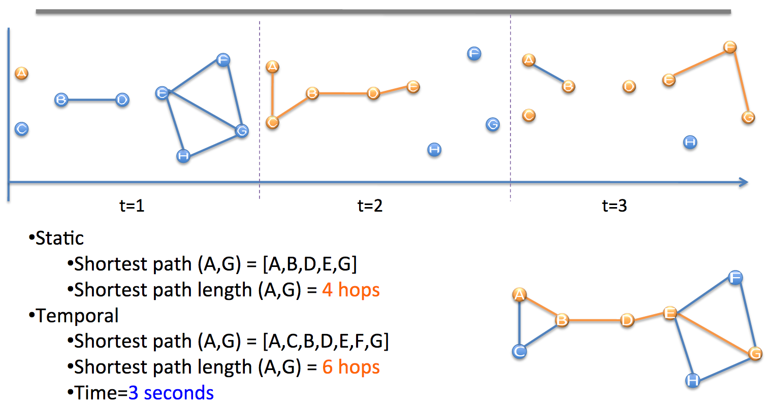
See the following example from Mascolo (2013). If it is a static network (the lower-right corner), the shortest path between A and G is [A, B, D, E, G]. When we consider the temporal network (see the time-sliced network above), A needs to go through C at time 2 in order to reach G; at time 3, the direct path between E and G is no longer available and E needs to go through F to reach G. As a result, the temporal shorted path between A and G becomes [A, C, B, D, E, F, G].
This is just one example concept that requires reconsideration in temporal networks.
11.1.1 Tools for temporal network analysis
R
R packages networkDynamic, tsna, and ndtv are very useful for temporal network analysis and visualization.
If you are interested, check out this amazing tutorial about Temporal Network Analysis with R.
You can download this demo R script I created based on the tutorial and reproduce the analysis. Note the dynamic network visualization you saw above was created from this tutorial.
Gephi
Gephi also supports the analysis of dynamic networks. This tutorial provides a useful introduction. See also the Youtube video below, if you use Gephi.
11.2 Week 11 Activities and Upcoming Milestones
11.2.1 Read, Annotate, and Explore
Read Blonder et al. (2012) – link.
Our textbook does not have a chapter on this topic. Please note this paper is from ecology and evolutionary biology. So please focus on the methods explained in the paper.Annotate as we normally do using proper hashtags (e.g.,
question,idea,stats) and doing ourABCs(i.e., “Ask a question”, “Brag about your understanding”, and “Connect another peer’s ideas”). Build community knowledge: Because this week’s topic is of great complexity, we’re going to rely on our collective wisdom to develop deeper understanding. So please seek additional resources on your own, share back via Hypothesis or Slack, and help out a colleague.
Optional: You’re also encouraged to explore additional resources and examples of temporal SNA by yourself. Below are a few readings you can start with:
- Gloor et al. (2004)
- Paranjape, Benson, and Leskovec (2017)
- Jiang et al. (2013)
- Myllari, Ahlberg, and Dillon (2010)
- Rodriguez et al. (2014)
- Raghavan et al. (2014)
- Carley et al. (2014)
Have a wonderful week!
References
Blonder, Benjamin, Tina W Wey, Anna Dornhaus, Richard James, and Andrew Sih. 2012. “Temporal Dynamics and Network Analysis.” Methods in Ecology and Evolution / British Ecological Society 3 (6): 958–72. https://doi.org/10.1111/j.2041-210X.2012.00236.x.
Carley, Kathleen M, Jürgen Pfeffer, Fred Morstatter, and Huan Liu. 2014. “Embassies Burning: Toward a Near-Real-Time Assessment of Social Media Using Geo-Temporal Dynamic Network Analytics.” Social Network Analysis and Mining 4 (1): 195. https://doi.org/10.1007/s13278-014-0195-3.
Gloor, P, Rob Laubacher, Yan Zhao, and S Dynes. 2004. “Temporal Visualization and Analysis of Social Networks.” In NAACSOS Conference, June, 27–29. Citeseer.
Jiang, Feng, Jiemin Wang, Abram Hindle, and Mario A Nascimento. 2013. “Mining the Temporal Evolution of the Android Bug Reporting Community via Sliding Windows.” CoRR abs/1310.7.
Mascolo, Cecilia. 2013. Temporal Social Network Metrics and Applications.
Myllari, J, M Ahlberg, and P Dillon. 2010. “The Dynamics of an Online Knowledge Building Community: A 5-Year Longitudinal Study.” British Journal of Educational Technology: Journal of the Council for Educational Technology 41 (3): 365–87. https://doi.org/10.1111/j.1467-8535.2009.00972.x.
Paranjape, Ashwin, Austin R. Benson, and Jure Leskovec. 2017. “Motifs in Temporal Networks.” In Proceedings of the Tenth ACM International Conference on Web Search and Data Mining, 601–10. WSDM ’17. New York, NY, USA: Association for Computing Machinery. https://doi.org/10.1145/3018661.3018731.
Raghavan, V, G Ver Steeg, A Galstyan, and A G Tartakovsky. 2014. “Modeling Temporal Activity Patterns in Dynamic Social Networks.” IEEE Transactions on Computational Social Systems 1 (1): 89–107. https://doi.org/10.1109/TCSS.2014.2307453.
Rodriguez, Manuel Gomez, Jure Leskovec, David Balduzzi, and Bernhard Schölkopf. 2014. “Uncovering the Structure and Temporal Dynamics of Information Propagation.” Network Science 2 (1): 26–65. https://doi.org/10.1017/nws.2014.3.
Schelling, Thomas C. 1969. “Models of Segregation.” The American Economic Review 59 (2): 488–93.