Principal Componants Analysis
Setup
intall libraries
Run PCA
Prep data and run PCA
x<-pp_all_Met_wide
x<-x[-c(1,3)]
x<-distinct(x)

rownames(x)<-x[,1]
x<-x[-c(1)]

x$pp_area<-as.numeric(x$pp_area)
x$pp_area<-as.numeric(x$dist2cent)

x[is.na(x)]<-0

#create grouping variable
x$area_group <- cut(x$pp_area, 4)

# x.pca<-prcomp(x[,c(8, 11:27)], center = TRUE, scale. = TRUE)
# summary(x.pca)

x.pca<-princomp(x[,c(4:5, 8:9, 11:27)], cor=TRUE)
summary(x.pca)
print(x.pca$loadings)
save(x.pca, file="3_pipeline/tmp/x.pca.rData")

x.pca$scores

#save output as a txt file
sink("4_output/PCA/summary_pca.txt")
print(summary(x.pca))
sink()

# x.pca_2<-princomp(x[,c(8:9, 11:57)], cor=TRUE)
# summary(x.pca_2)

x.pca<-princomp(x[,c(4:5, 8:9, 11:27)], cor=TRUE)
# summary(x.pca_2)
##
## Loadings:
## Comp.1 Comp.2 Comp.3 Comp.4 Comp.5 Comp.6 Comp.7 Comp.8 Comp.9
## cur_in_mean 0.216 0.225 0.480 0.444 0.580
## cur_diff -0.150 -0.354 -0.199 0.384
## slope_mean 0.245 -0.198 -0.341 -0.149 0.465
## dist2cent -0.204 0.124 0.394 0.252 -0.157
## trail_proportion 0.153 -0.301 -0.113 -0.196 0.398 0.118 0.232
## trail_tot_buf -0.336 0.400 0.212 0.123
## road_proportion -0.141 -0.269 -0.270 -0.410 -0.199 -0.191 0.490
## road_tot_buf -0.157 -0.397 0.343 0.221 0.124
## canopy_grass -0.155 0.167 -0.337 -0.129 -0.384 -0.148 0.155
## canopy_shrub_con -0.255 0.415 0.227 0.332 -0.180
## canopy_shrub_dec 0.127 -0.118 0.332 -0.203 0.397 -0.458 0.150
## canopy_tree_con 0.368 -0.184 -0.167 -0.102
## canopy_tree_dec 0.374 -0.205 -0.160
## PRIMECLASS_NVE -0.296 -0.422 0.131
## PRIMECLASS_VEG 0.296 0.421 -0.132
## LANDCLAS_DEV -0.338 -0.253 -0.156 0.307 0.186 -0.123
## LANDCLAS_MOD -0.229 0.382 -0.243
## LANDCLAS_NAT -0.244 0.137 0.213 -0.578 0.245 -0.272
## LANDCLAS_NAW 0.386 -0.115 0.316 -0.110
## LANDCLAS_NNW 0.178 0.213 0.269 -0.313 -0.441 0.147
## LANDCLAS_WET 0.206 0.231 0.180 0.139 -0.596 0.524
## Comp.10 Comp.11 Comp.12 Comp.13 Comp.14 Comp.15 Comp.16
## cur_in_mean 0.282 0.130 0.110
## cur_diff -0.315 -0.257 -0.467 0.189 -0.127
## slope_mean -0.286 0.327 0.164 -0.190
## dist2cent -0.584 -0.296 -0.483
## trail_proportion -0.395 -0.187 -0.398 0.150 -0.430 -0.183 0.118
## trail_tot_buf -0.268 0.480 0.166 -0.257 0.367 -0.345
## road_proportion 0.271 -0.306 0.351
## road_tot_buf 0.283 0.161 0.157 -0.135 -0.110 -0.586 0.333
## canopy_grass 0.252 0.416 0.331 -0.345 -0.359
## canopy_shrub_con 0.282 -0.302 -0.423 0.332 0.274 -0.123
## canopy_shrub_dec -0.140 -0.479 0.283 0.202 0.161 -0.141
## canopy_tree_con 0.229 -0.193 -0.189 0.124 -0.154 -0.358
## canopy_tree_dec 0.176 -0.209 -0.144 0.124 -0.168 -0.297
## PRIMECLASS_NVE 0.114
## PRIMECLASS_VEG -0.114
## LANDCLAS_DEV -0.106 0.151 -0.127 0.164
## LANDCLAS_MOD 0.111 -0.292 -0.351 -0.146
## LANDCLAS_NAT 0.242 -0.132 0.189
## LANDCLAS_NAW 0.226 0.267
## LANDCLAS_NNW -0.112 0.316 -0.446 0.304
## LANDCLAS_WET -0.259 -0.106 0.305 -0.108
## Comp.17 Comp.18 Comp.19 Comp.20 Comp.21
## cur_in_mean
## cur_diff 0.446
## slope_mean -0.531
## dist2cent 0.123
## trail_proportion
## trail_tot_buf
## road_proportion 0.214
## road_tot_buf
## canopy_grass 0.156
## canopy_shrub_con
## canopy_shrub_dec
## canopy_tree_con -0.203 -0.670
## canopy_tree_dec -0.124 0.736
## PRIMECLASS_NVE -0.109 -0.513 -0.635
## PRIMECLASS_VEG 0.106 -0.649 -0.496
## LANDCLAS_DEV -0.207 -0.349 0.637
## LANDCLAS_MOD -0.320 -0.239 0.562
## LANDCLAS_NAT 0.144 -0.237 0.437
## LANDCLAS_NAW 0.418 -0.249 0.581
## LANDCLAS_NNW -0.133 0.309
## LANDCLAS_WET
##
## Comp.1 Comp.2 Comp.3 Comp.4 Comp.5 Comp.6 Comp.7 Comp.8 Comp.9
## SS loadings 1.000 1.000 1.000 1.000 1.000 1.000 1.000 1.000 1.000
## Proportion Var 0.048 0.048 0.048 0.048 0.048 0.048 0.048 0.048 0.048
## Cumulative Var 0.048 0.095 0.143 0.190 0.238 0.286 0.333 0.381 0.429
## Comp.10 Comp.11 Comp.12 Comp.13 Comp.14 Comp.15 Comp.16 Comp.17
## SS loadings 1.000 1.000 1.000 1.000 1.000 1.000 1.000 1.000
## Proportion Var 0.048 0.048 0.048 0.048 0.048 0.048 0.048 0.048
## Cumulative Var 0.476 0.524 0.571 0.619 0.667 0.714 0.762 0.810
## Comp.18 Comp.19 Comp.20 Comp.21
## SS loadings 1.000 1.000 1.000 1.000
## Proportion Var 0.048 0.048 0.048 0.048
## Cumulative Var 0.857 0.905 0.952 1.000Visualize eigenvalues (scree plot).
How much variance is explained by each principal componant?
png("4_output/PCA/scree_plot", width=1000, height=600)
fviz_eig(x.pca)
dev.off()

# Contributions of variables to PC1
png("4_output/PCA/cont_PCA1_plot", width=1000, height=600)
fviz_contrib(x.pca, choice = "var", axes = 1, top = 10)
dev.off()


# Contributions of variables to PC2
png("4_output/PCA/cont_PCA2_plot", width=1000, height=600)
fviz_contrib(x.pca, choice = "var", axes = 2, top = 10)
dev.off()
Figure 4.1: Scree plot showing how much variance is explained by each PCA
Figure 4.2: Contribution of variables to Dim-1
Figure 4.3: Contribution of variables to Dim-2
Plot results
# create ggplot theme
custom_theme<-function(){theme(
        panel.background = element_rect(fill = "white", color="#636363"),
        # axis.line.y = element_line(colour = "#636363"),
        axis.text.y = element_text(colour="#636363"),
        axis.ticks.y = element_line(colour = "#636363"),
        axis.title.y = element_text(colour="#636363"),
        axis.text.x = element_text(colour="#636363"),
        axis.ticks.x = element_line(colour = "#636363"),
        #axis.line.x = element_line(colour = "#636363"),
        axis.title.x = element_text(colour="#636363"),
        legend.title = element_text(colour="#636363"),
        legend.text = element_text(colour="#636363"),
        legend.key = element_rect(fill = "white"),
      panel.grid.major = element_line(size = 0.0, colour="#bdbdbd"),
        #panel.grid.minor = element_line(size = 0.0)
        )}


# with labels
ggbiplot(x.pca, circle = TRUE)+
  custom_theme()
ggsave(filename="4_output/PCA/pca.png",  width = 13, height = 10)


#current difference
ggbiplot(x.pca,  ellipse=TRUE, groups=x$cur_diff_group)+
  labs(color="current difference")+
    custom_theme()
ggsave(filename="4_output/PCA/pca_cur_diff_group.png",  width = 13, height = 10)


#mean current
ggbiplot(x.pca,  ellipse=TRUE, groups=x$cur_in_mean_group)+
  labs(color="RoG reach")+
    custom_theme()
ggsave(filename="4_output/PCA/pca_cur_in_mean_group.png", width = 13, height = 10)


#distance 2 city center
ggbiplot(x.pca,  ellipse=TRUE, groups=x$dist2cent_group)+
  labs(color="distance to city center")+
    custom_theme()
ggsave(filename="4_output/PCA/pca_dist2cent_group.png", width = 13, height = 10)


#reach
ggbiplot(x.pca,  ellipse=TRUE, groups=x$Reach)+
  labs(color="RoG reach")+
    custom_theme()
ggsave(filename="4_output/PCA/pca_Reach_group.png", width = 13, height = 10)


#polygon area
ggbiplot(x.pca,  ellipse=TRUE, groups=x$area_group)+
  labs(color="pinch-point area (m)")+
    custom_theme()
ggsave(filename="4_output/PCA/pca_area_group.png", width = 13, height = 10)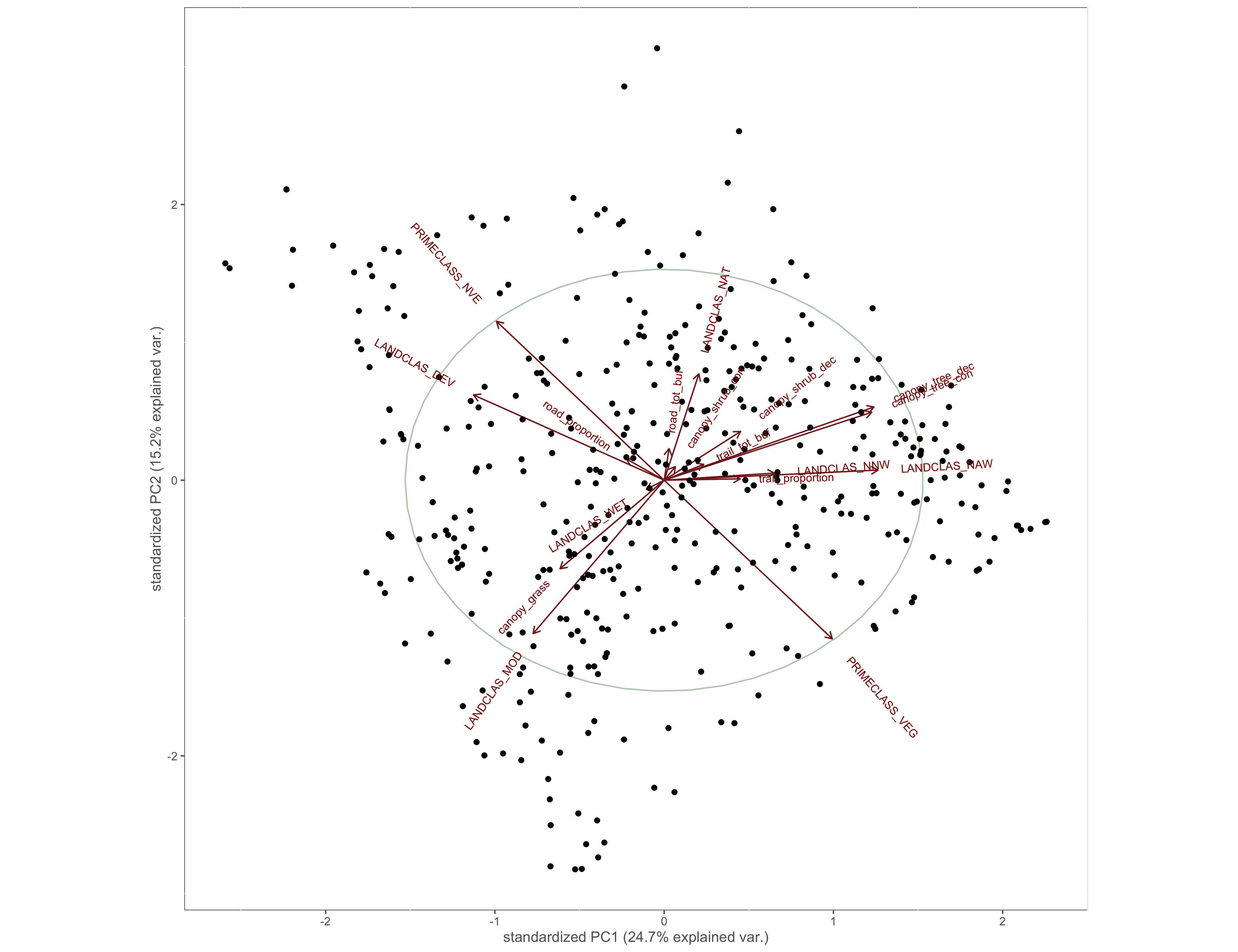
Figure 4.4: PCA results
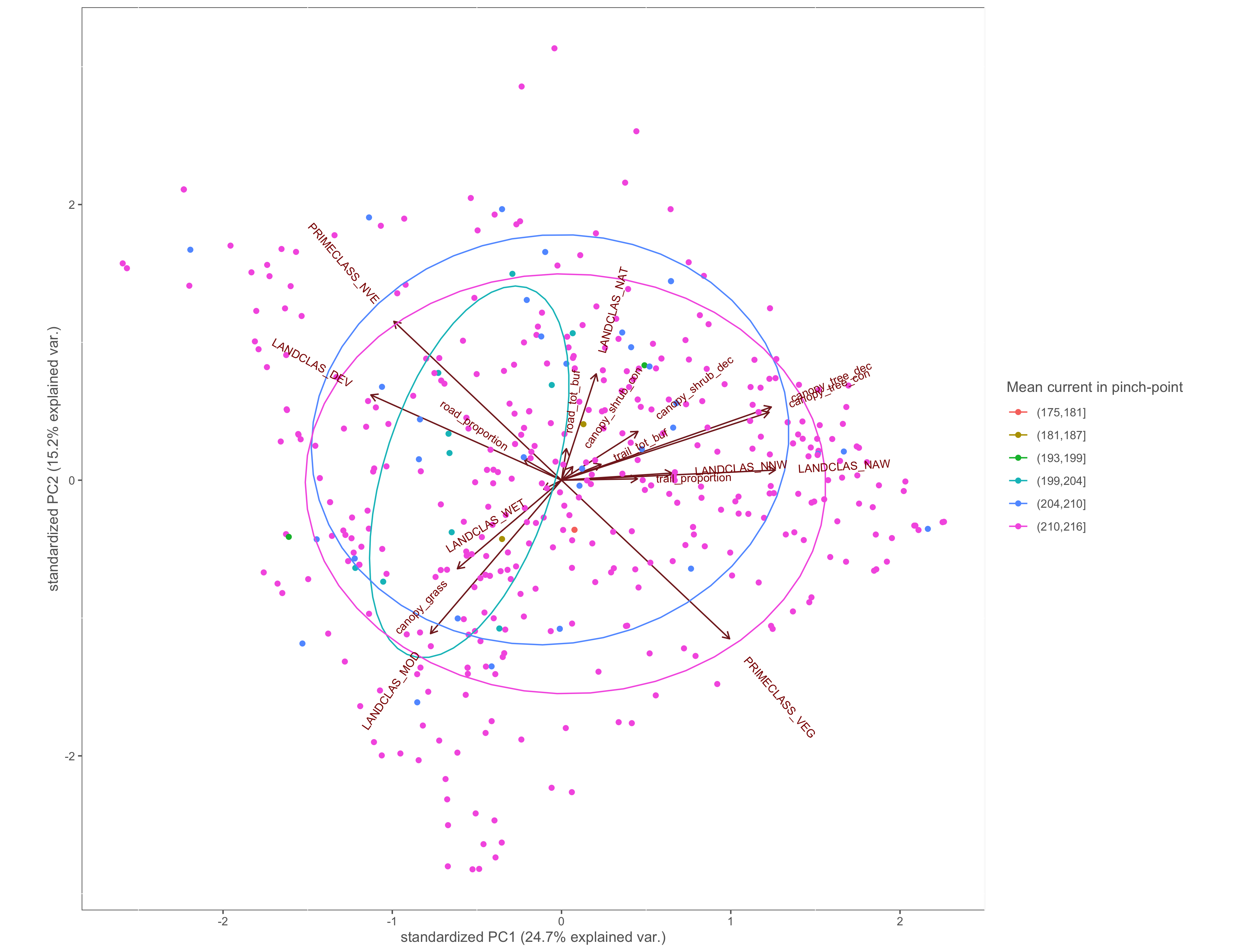
Figure 4.5: PCA biplot with pinch-points grouped by the within pinch-pont mean current values
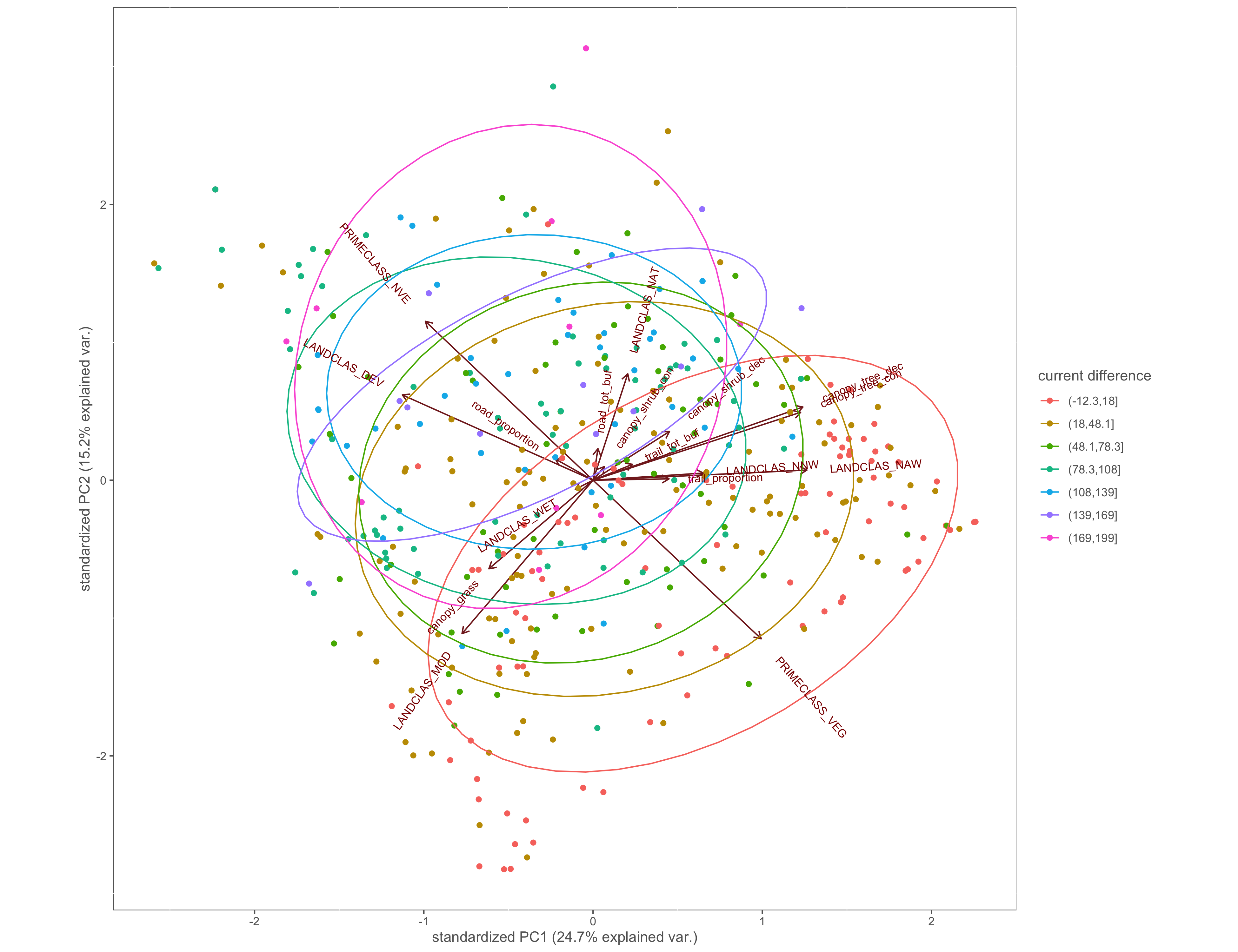
Figure 4.6: PCA biplot with pinch-points grouped by the difference between within and without current values
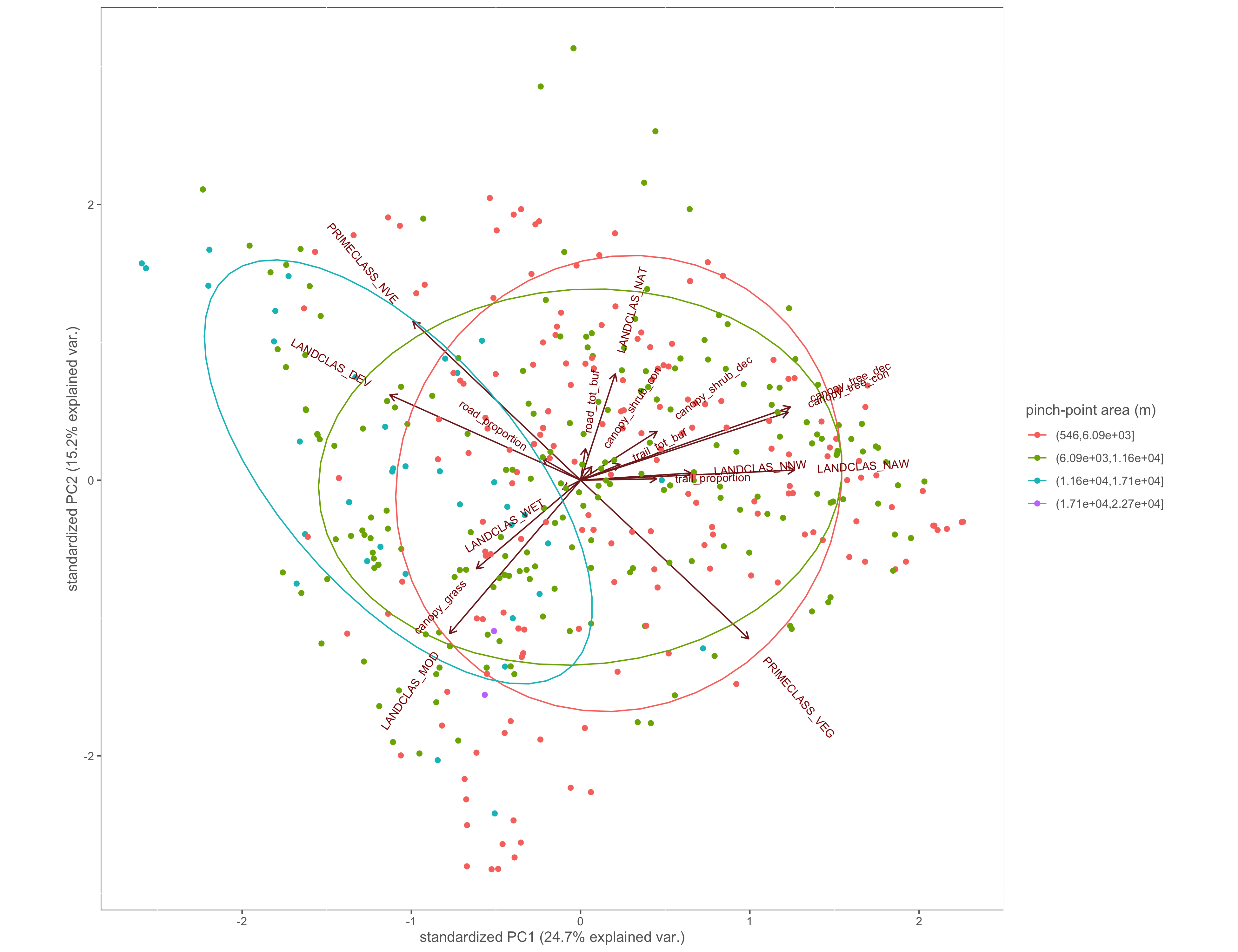
Figure 4.7: PCA biplot with pinch-points grouped by the pinch-point polygon area
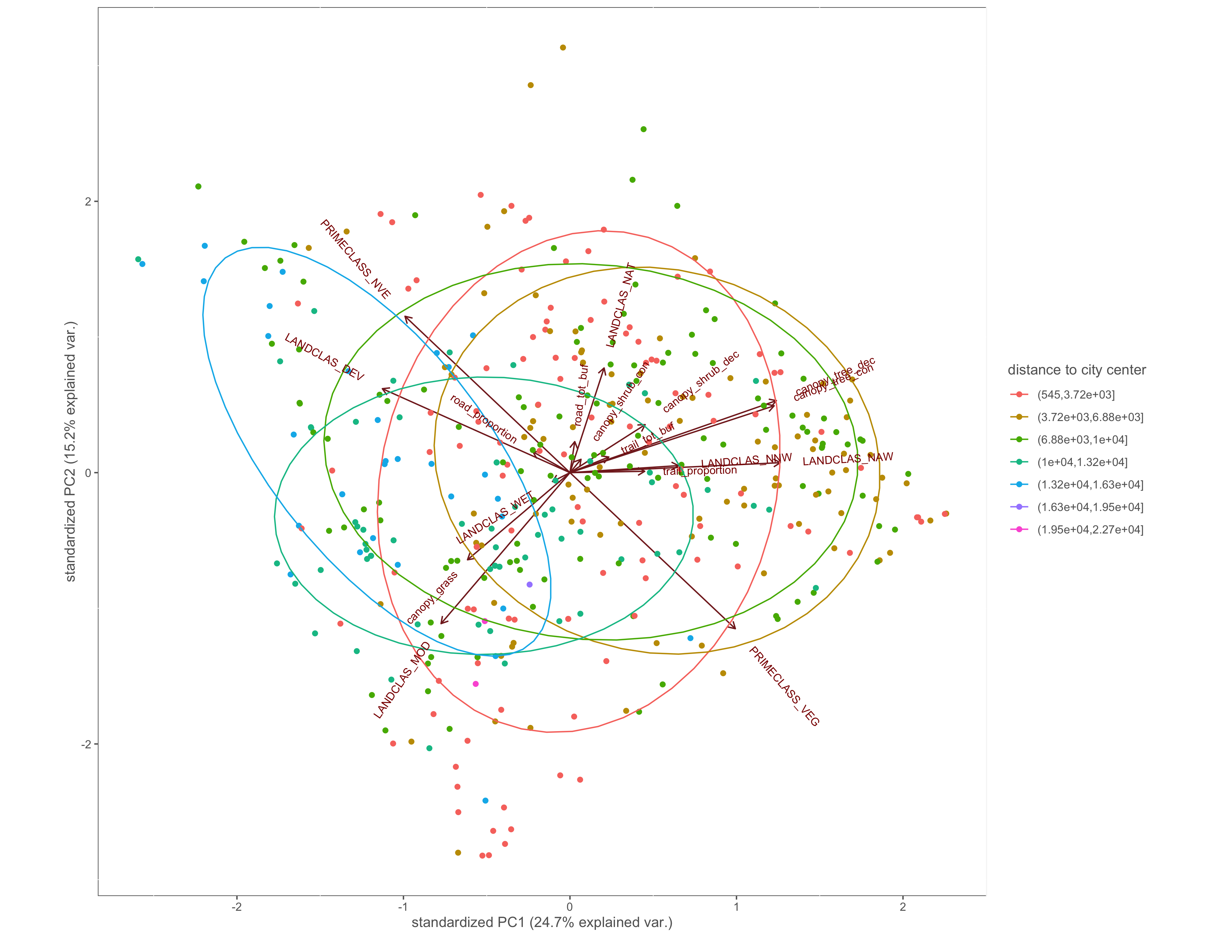
Figure 4.8: PCA biplot with pinch-points grouped by the distance to city center
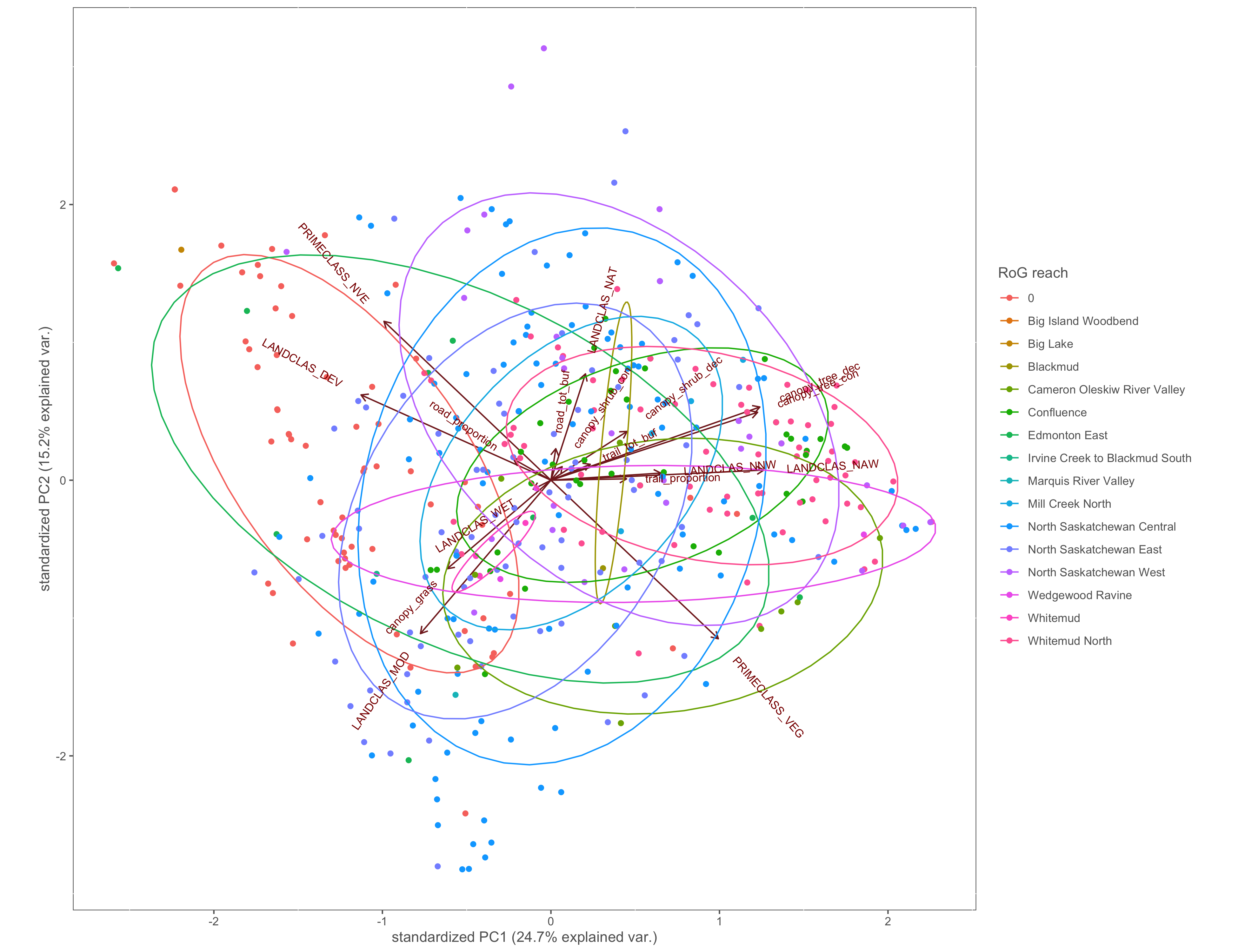
Figure 4.9: PCA biplot with pinch-points grouped by the RoG reach
hierarchical clustering of PCA
#hc<-hclust(dist(x.pca_2$loadings))

loadings = x.pca$loadings[]

    q = loadings[,1]
    y = loadings[,2]
    z = loadings[,3]


    hc = hclust(dist(cbind(q,y)), method = 'ward')

    png("4_output/PCA/hclust_plot", width=1000, height=600)
    plot(hc, axes=F,xlab='', ylab='',sub ='', main='Clusters')
    rect.hclust(hc, k=3, border='red')
    dev.off()


# view clusters in biplot
x.pca2<-x.pca

# pct=paste0(colnames(x.pca2$x)," (",sprintf("%.1f",x.pca2$sdev/sum(x.pca2$sdev)*100),"%)")
p2=as.data.frame(x.pca2$x)


x.pca2$k=factor(cutree(hclust(dist(x), method='complete'  ),k=10))
ggbiplot(x.pca2,  ellipse=TRUE, groups=x.pca2$k)+
  labs(color="cluster")+
    custom_theme()
Figure 4.10: Hierarchical clusters of PCA variables