Chapter 6 Text as Data
6.1 Our Scraped Corpus
#Step 2: Clean Text
df <- raw %>%
  mutate(
    text=tolower(text),
    text=str_remove_all(text,"[:punct:]"),
    text=str_remove_all(text,"[:digit:]"),
    opinion=case_when(
      str_detect(title,"Opinion")~1,
      TRUE~0
    )
)## Joining, by = "word"#Step 5: Visualize Text
tidy_counts %>%
mutate(opinion = as.factor(opinion)) %>%
group_by(opinion) %>%
top_n(50) %>%
ggplot(aes(label=word, size=n))+
geom_text_wordcloud(aes(color=opinion),
size = 4) +
scale_size_area(max_size = 5) +
theme_minimal()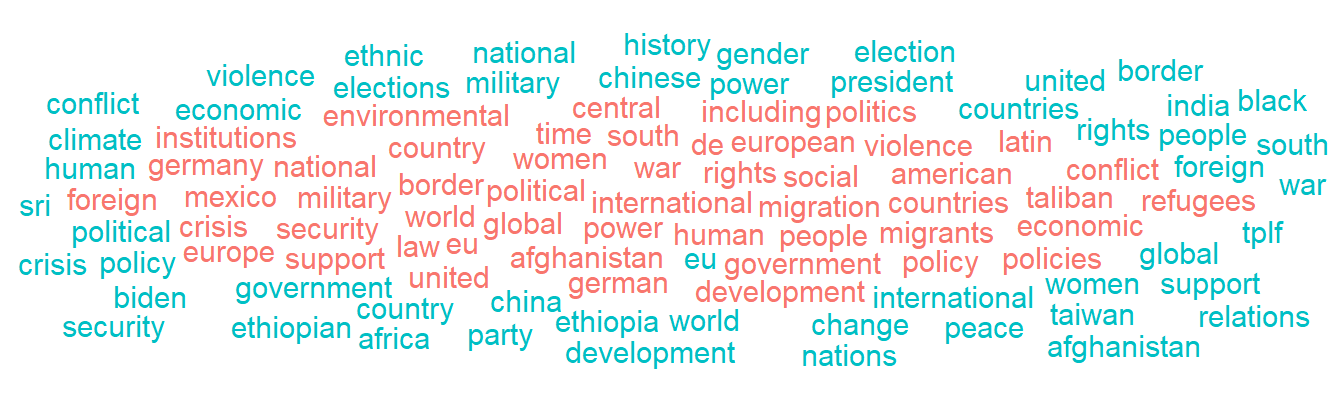
Figure 6.1: A Tidy Wordcloud
tidy_counts %>%
  head(20) %>%
  ggplot()+
  geom_col(aes(n,reorder(word, n)))+
  theme_minimal()+
  labs(x=NULL,y="Top Words E-IR")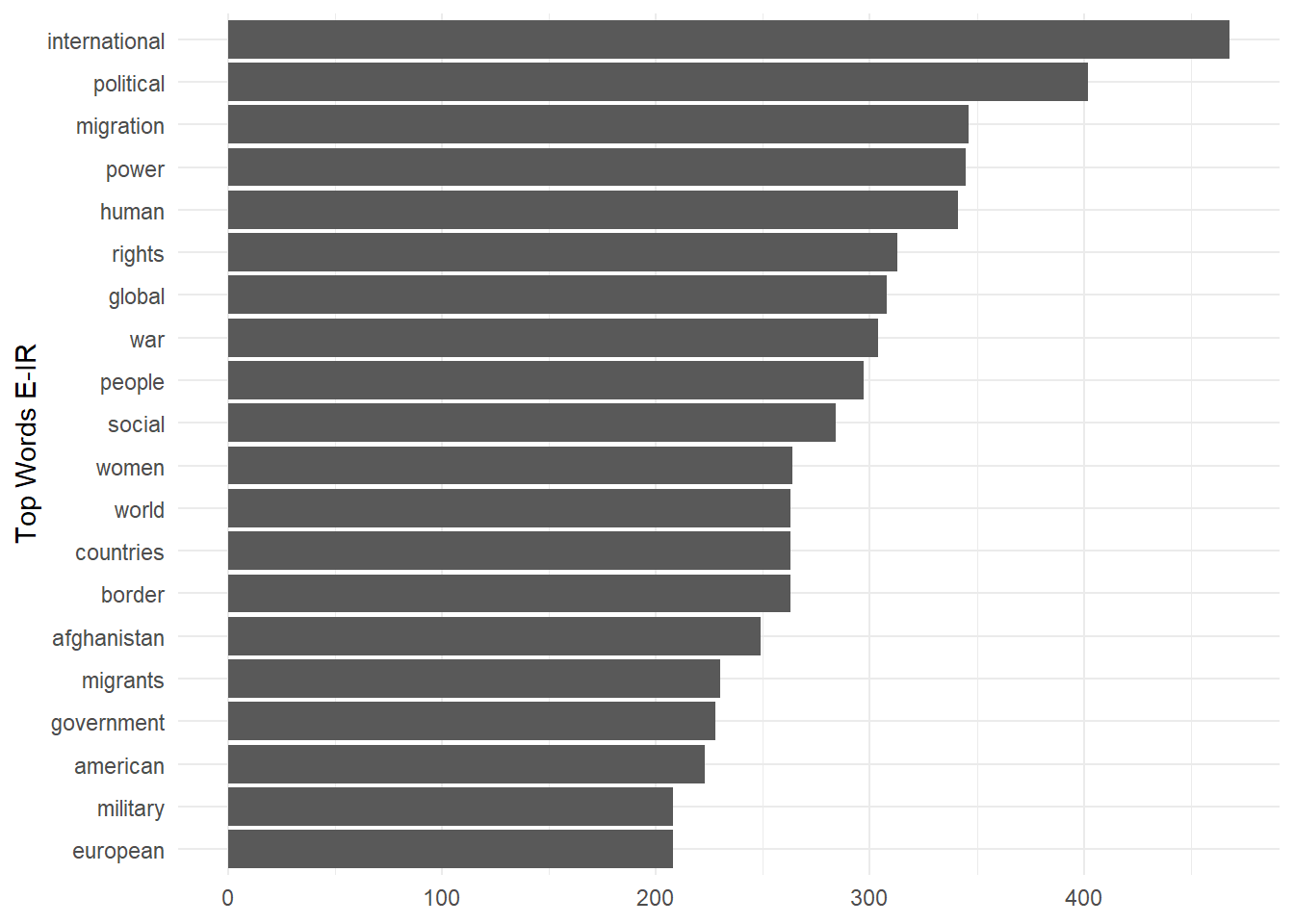
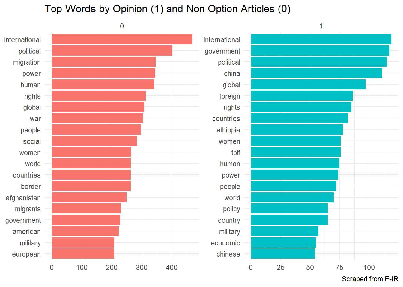
tidy_counts %>%
  mutate(opinion = as.factor(opinion)) %>%
  group_by(opinion) %>%
  top_n(20) %>%
  ggplot()+
  geom_col(aes(x = n,
               y = reorder_within(word, n, opinion),
               fill = opinion),
           show.legend = F)+
  theme_minimal()+
  scale_y_reordered() +
  facet_wrap(~opinion,
             scales = "free")+
  labs(x = NULL,
       y = NULL,
       title = "Top Words by Opinion (1) and Non Option Articles (0)",
       caption = "Scraped from E-IR")