Chapter 4 R Markdown Reports

4.1 Basic Syntax

You can do many things with Markdown, from reports to blog post and even books with bookdown. Here we will cover the 20% of elements that will be useful 80% of the time!¹

We can change the fonts (i.e., bold *text* or italics **text**), as well as make headers and bullet points to make our reports tidier. For example:

For bullets point we write: * Our Text
- For sub-items we write: + Our Text
For headers we write #s in front of our text depending on the hierarchy
- Header 2 is ## Header 2
- Header 3 is ### Header 3
- Header 4 is #### Header 4
For links (e.g., CheatSheet) we write: [text](url)
For footnotes we write: [^id] where you want the reference and [^id]: Footnote content preferably at the end of our document

4.1.1 Chunks

We put chunks inside our Markdown document to display various types of content such as code, outputs, results, and figures. This is similar to the scripts we have been using thus far. In RStudio, you can run chunks individually. Each chunk must have its own name. The basic syntax of chunks is as follows: ```{r name, options} #content ```

4.1.2 Display Options

Chunks have several options that will determine how you want them to appear in your reports. Code can run, but be hidden, it can be shown but not run, or you can show the output but hide the code. You can type these options into the script or click the settings button in each chunk in RStudio. Here are some common examples:

Option	Default	Effect
`eval`	TRUE	Whether to evaluate the code and include its results
`echo`	TRUE	Whether to display code along with its results
`warning`	TRUE	Whether to display warnings
`error`	FALSE	Whether to display errors
`message`	TRUE	Whether to display messages

4.1.2.1 In-line Code

We can also include in-line code to highlight objects (e.g., df) using the syntax: ` content `. Additionally, we can put console outputs in our text using the syntax: ` r content `. This will help us make our reporting more streamlined!

4.1.3 Tables

We can include HTML type tables in our reports using the syntax:

Col1     | Col2            
------- -|-----------
cell1.1  | cell1.2 
cell2.1  | cell2.2

For example, markdown syntax:

Variable      | Description             | Loading
--------------|-------------------------|--------------
`i1_singleb`  | Single Bidding Rate     | **Negative**
`i2_bnr`      | Trimmed Bidder Number   | **Positive**
`i3_max_msh`  | Market Concentration    | **Negative**
`i4_entryr`   | New Winner Rate         | **Positive**

Will output:

Variable	Description	Loading
`i1_singleb`	Single Bidding Rate	Negative
`i2_bnr`	Trimmed Bidder Number	Positive
`i3_max_msh`	Market Concentration	Negative
`i4_entryr`	New Winner Rate	Positive

You can include HTML code directly in the .rmd file. For example, if you write <br /> in the script you will get a new line in the knitted HTML.

4.2 Example with `mtcars` (yes, again…)

An R Markdown file in RStudio will include a setup chunk as the first chunk by default! This chunk is not included in the report (i.e., {r setup, include=FALSE}).

Now lets set up our own chunk. We can use this to load the libraries and data we need and to do some general cleaning of our mtcars data set.

In this example, we will use two libraries: stargazer and tidyverse. To avoid noisy output, we can change some chunk parameters to silence warnings and messages: {r first_chunk, echo=TRUE, message=FALSE, warning=FALSE}.

library(tidyverse)
library(stargazer)
df <- mtcars

# You can make comments inside chunks, just as in R scripts
df$model <- row.names(df)
df[df$am == 1,]$am <- "Manual"
df[df$am == 0,]$am <- "Automatic"
df$am <- as.factor(df$am)
df$cyl <- as.factor(df$cyl)

Let’s explore the structure of our data set df but omit the code used to retrieve it.

## 'data.frame':    32 obs. of  12 variables:
##  $ mpg  : num  21 21 22.8 21.4 18.7 18.1 14.3 24.4 22.8 19.2 ...
##  $ cyl  : Factor w/ 3 levels "4","6","8": 2 2 1 2 3 2 3 1 1 2 ...
##  $ disp : num  160 160 108 258 360 ...
##  $ hp   : num  110 110 93 110 175 105 245 62 95 123 ...
##  $ drat : num  3.9 3.9 3.85 3.08 3.15 2.76 3.21 3.69 3.92 3.92 ...
##  $ wt   : num  2.62 2.88 2.32 3.21 3.44 ...
##  $ qsec : num  16.5 17 18.6 19.4 17 ...
##  $ vs   : num  0 0 1 1 0 1 0 1 1 1 ...
##  $ am   : Factor w/ 2 levels "Automatic","Manual": 2 2 2 1 1 1 1 1 1 1 ...
##  $ gear : num  4 4 4 3 3 3 3 4 4 4 ...
##  $ carb : num  4 4 1 1 2 1 4 2 2 4 ...
##  $ model: chr  "Mazda RX4" "Mazda RX4 Wag" "Datsun 710" "Hornet 4 Drive" ...

We can display code that we want to show case so our audience can reproduce our studies. Below, we mutate miles per gallon to kilometers per liter.

df <- df %>%
  mutate(kml = mpg / 2.352)

4.2.0.1 More Tables

We can also include some nice summary and regression tables using stargazer. Here we include the the summary statistics of our df. We can output the text that would show up in our console:

stargazer(df, type = "text", title="Descriptive Statistics", digits=1)

## 
## Descriptive Statistics
## =======================================================
## Statistic N  Mean  St. Dev. Min  Pctl(25) Pctl(75) Max 
## -------------------------------------------------------
## mpg       32 20.1    6.0     10    15.4     22.8    34 
## disp      32 230.7  123.9    71   120.8     326    472 
## hp        32 146.7   68.6    52    96.5     180    335 
## drat      32  3.6    0.5    2.8    3.1      3.9    4.9 
## wt        32  3.2    1.0    1.5    2.6      3.6    5.4 
## qsec      32 17.8    1.8    14.5   16.9     18.9   22.9
## vs        32  0.4    0.5     0      0        1      1  
## gear      32  3.7    0.7     3      3        4      5  
## carb      32  2.8    1.6     1      2        4      8  
## kml       32  8.5    2.6    4.4    6.6      9.7    14.4
## -------------------------------------------------------

Or we can output an HTML table by including the following options in our chunk: results='asis', message = FALSE. If you want to knit PDF files, you must put the type="latex" option in the stargazer command. The df must be a data.frame class object to work with the stargazer package.

**Descriptive Statistics**

Statistic	N	Mean	St. Dev.	Min	Pctl(25)	Pctl(75)	Max

mpg	32	20	6	10	15.4	22.8	34
disp	32	231	124	71	120.8	326	472
hp	32	147	69	52	96.5	180	335
drat	32	4	1	3	3	4	5
wt	32	3	1	2	3	4	5
qsec	32	18	2	14	17	19	23
vs	32	0	1	0	0	1	1
gear	32	4	1	3	3	4	5
carb	32	3	2	1	2	4	8
kml	32	9	3	4	7	10	14

Finally, if you want to format more modern tables, you might consider the kableExtra package, which allows you to display HTML friendly tables. You can choose many aesthetic options with the kable_styling() command. Below, we can see the entire df printed out inside a scroll box. We can set this and other parameters with functions from the kableExtra package.

library(kableExtra)

df %>% 
  kable(digits = 2,
      caption = "MT Cars Data") %>% 
  kable_styling() %>% 
  scroll_box(width = "100%", height = "300px")

Table 4.1: MT Cars Data
	mpg	cyl	disp	hp	drat	wt	qsec	vs	am	gear	carb	model	kml
Mazda RX4	21.0	6	160.0	110	3.90	2.62	16.46	0	Manual	4	4	Mazda RX4	8.93
Mazda RX4 Wag	21.0	6	160.0	110	3.90	2.88	17.02	0	Manual	4	4	Mazda RX4 Wag	8.93
Datsun 710	22.8	4	108.0	93	3.85	2.32	18.61	1	Manual	4	1	Datsun 710	9.69
Hornet 4 Drive	21.4	6	258.0	110	3.08	3.21	19.44	1	Automatic	3	1	Hornet 4 Drive	9.10
Hornet Sportabout	18.7	8	360.0	175	3.15	3.44	17.02	0	Automatic	3	2	Hornet Sportabout	7.95
Valiant	18.1	6	225.0	105	2.76	3.46	20.22	1	Automatic	3	1	Valiant	7.70
Duster 360	14.3	8	360.0	245	3.21	3.57	15.84	0	Automatic	3	4	Duster 360	6.08
Merc 240D	24.4	4	146.7	62	3.69	3.19	20.00	1	Automatic	4	2	Merc 240D	10.37
Merc 230	22.8	4	140.8	95	3.92	3.15	22.90	1	Automatic	4	2	Merc 230	9.69
Merc 280	19.2	6	167.6	123	3.92	3.44	18.30	1	Automatic	4	4	Merc 280	8.16
Merc 280C	17.8	6	167.6	123	3.92	3.44	18.90	1	Automatic	4	4	Merc 280C	7.57
Merc 450SE	16.4	8	275.8	180	3.07	4.07	17.40	0	Automatic	3	3	Merc 450SE	6.97
Merc 450SL	17.3	8	275.8	180	3.07	3.73	17.60	0	Automatic	3	3	Merc 450SL	7.36
Merc 450SLC	15.2	8	275.8	180	3.07	3.78	18.00	0	Automatic	3	3	Merc 450SLC	6.46
Cadillac Fleetwood	10.4	8	472.0	205	2.93	5.25	17.98	0	Automatic	3	4	Cadillac Fleetwood	4.42
Lincoln Continental	10.4	8	460.0	215	3.00	5.42	17.82	0	Automatic	3	4	Lincoln Continental	4.42
Chrysler Imperial	14.7	8	440.0	230	3.23	5.34	17.42	0	Automatic	3	4	Chrysler Imperial	6.25
Fiat 128	32.4	4	78.7	66	4.08	2.20	19.47	1	Manual	4	1	Fiat 128	13.78
Honda Civic	30.4	4	75.7	52	4.93	1.61	18.52	1	Manual	4	2	Honda Civic	12.93
Toyota Corolla	33.9	4	71.1	65	4.22	1.83	19.90	1	Manual	4	1	Toyota Corolla	14.41
Toyota Corona	21.5	4	120.1	97	3.70	2.46	20.01	1	Automatic	3	1	Toyota Corona	9.14
Dodge Challenger	15.5	8	318.0	150	2.76	3.52	16.87	0	Automatic	3	2	Dodge Challenger	6.59
AMC Javelin	15.2	8	304.0	150	3.15	3.44	17.30	0	Automatic	3	2	AMC Javelin	6.46
Camaro Z28	13.3	8	350.0	245	3.73	3.84	15.41	0	Automatic	3	4	Camaro Z28	5.65
Pontiac Firebird	19.2	8	400.0	175	3.08	3.85	17.05	0	Automatic	3	2	Pontiac Firebird	8.16
Fiat X1-9	27.3	4	79.0	66	4.08	1.94	18.90	1	Manual	4	1	Fiat X1-9	11.61
Porsche 914-2	26.0	4	120.3	91	4.43	2.14	16.70	0	Manual	5	2	Porsche 914-2	11.05
Lotus Europa	30.4	4	95.1	113	3.77	1.51	16.90	1	Manual	5	2	Lotus Europa	12.93
Ford Pantera L	15.8	8	351.0	264	4.22	3.17	14.50	0	Manual	5	4	Ford Pantera L	6.72
Ferrari Dino	19.7	6	145.0	175	3.62	2.77	15.50	0	Manual	5	6	Ferrari Dino	8.38
Maserati Bora	15.0	8	301.0	335	3.54	3.57	14.60	0	Manual	5	8	Maserati Bora	6.38
Volvo 142E	21.4	4	121.0	109	4.11	2.78	18.60	1	Manual	4	2	Volvo 142E	9.10

We can also include some results in line as well. For example, we know that our df has 32 observations and 13 variables. We can also report that the average weight of cars is 3.22 tons.

4.2.0.2 Figures

Finally, we can include plots as figures with several chunk options such as fig.cap, fig.align, and out.width.

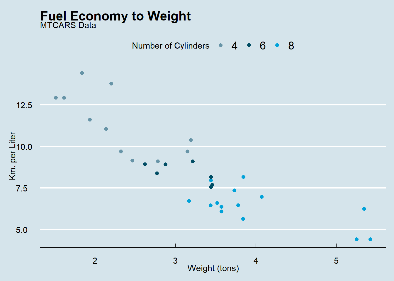
(#fig:figure_1)Figure 1: Scatter Plot

Our .rmd file takes the source file location (where it is saved) as the working directory when knitted. It will ignore anything in the working environment that is not within the markdown script, and all of the outputs will be in saved the the working directory. If it must read any inputs (e.g., read_csv()), the files should be in the same folder.

ggsave("cars_plot.png")

## Saving 7 x 5 in image

4.3 UNGA Network Example

4.3.1 Packages

library(kableExtra)
library(tidyverse)
library(countrycode)
library(reshape2)
library(tidytext)
library(sf)
library(rnaturalearth)
library(ggraph)
library(tidygraph)
library(countrycode)
library(stargazer)
library(broom)
library(DiagrammeR)
library(DiagrammeRsvg)  
library(rsvg)  
cache = T
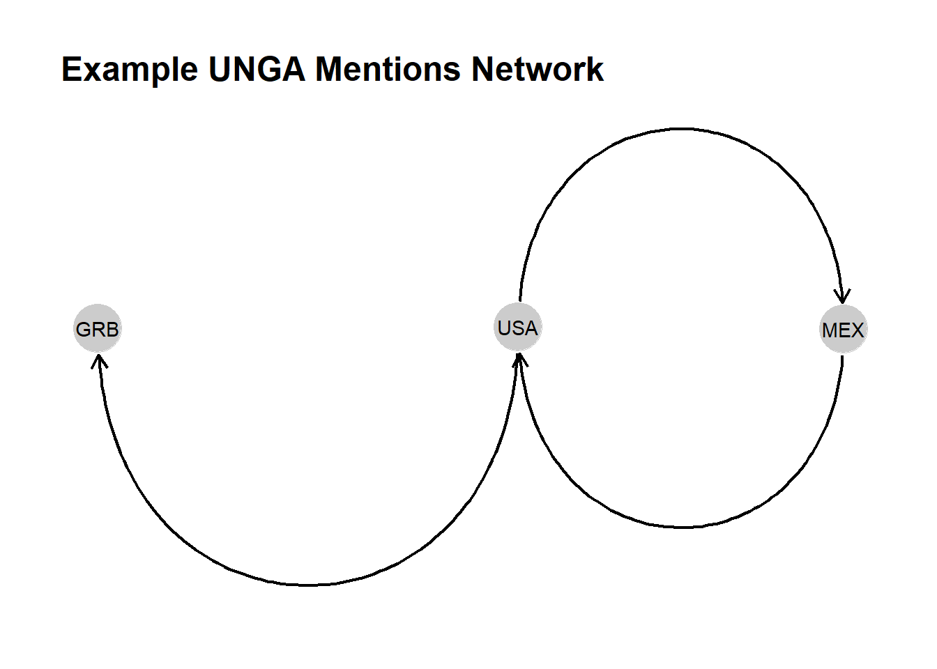
set.seed(42)

4.3.2 Proof of Concept

example <- data.frame(
  country = c("GRB","MEX", "USA"),
  year = c(2016, 2016, 2017),
  text = c("London is the capital of the United Kingdom.", 
           "The capital of Mexico is Mexico City and the capital of the United States is Washington.",
           "The Great Britain, Mexico and the United States are members of the UN."
  )
)

new_vars = c("GRB","MEX", "USA", "FRA")

example <- 
  cbind(example, setNames(lapply(new_vars, function(x) x=NA), new_vars))

code_list_df <- data.frame(
  country = c("GRB","MEX", "USA", "FRA"),
  country_ids = c("Great Britain|United Kingdom",
                  "Mexico",
                  "United States|USA|United States of America",
                  "France")
)

for(i in 1:nrow(example)) {
  
  for(j in 1:nrow(code_list_df)){
    
    example[i,code_list_df[[j,"country"]]] <- 
      str_count(example$text[i], code_list_df[[j,"country_ids"]])
    
    }
    
}

(#tab:data_frame_example)Example Data
country	year	text	GRB	MEX	USA
GRB	2016	London is the capital of the United Kingdom.	1	0	0
MEX	2016	The capital of Mexico is Mexico City and the capital of the United States is Washington.	0	2	1
USA	2017	The Great Britain, Mexico and the United States are members of the UN.	1	1	1

4.4 Troubleshooting

You may encounter that code that works just fine in the scripts, does not knit when you put it in a Markdown file. There are several possible reasons for this:

Markdown starts a new session, so it will ignore objects like a df in the environment.
Make sure to explicitly load your data in a chunk!

Data Visualization for International Relations

4.1 Basic Syntax

Header 2 is `## Header 2`

Header 3 is `### Header 3`

Header 4 is `#### Header 4`

4.1.1 Chunks

4.1.2 Display Options

4.1.2.1 In-line Code

4.1.3 Tables

4.2 Example with `mtcars` (yes, again…)

4.2.0.1 More Tables

4.2.0.2 Figures

4.3 UNGA Network Example

4.3.1 Packages

4.3.2 Proof of Concept

4.4 Troubleshooting

Chapter 4 R Markdown Reports

4.1 Basic Syntax

Header 2 is ## Header 2

Header 3 is ### Header 3

Header 4 is #### Header 4

4.1.1 Chunks

4.1.2 Display Options

4.1.2.1 In-line Code

4.1.3 Tables

4.2 Example with mtcars (yes, again…)

4.2.0.1 More Tables

4.2.0.2 Figures

4.3 UNGA Network Example

4.3.1 Packages

4.3.2 Proof of Concept

4.4 Troubleshooting

Header 2 is `## Header 2`

Header 3 is `### Header 3`

Header 4 is `#### Header 4`

4.2 Example with `mtcars` (yes, again…)