micro_sbatch(
  work_dir = "~/test_project", step = "fastp",
  all_sample_num = 40, array = 1, partition = "cpu",
  cpus_per_task = 1, mem_per_cpu = "2G"
)11 Other features
In addition to its core functionalities, pctax provides several auxiliary functions to streamline downstream bioinformatics workflows. For instance, it includes a built-in metagenomic workflow that simplifies the analysis of metagenomic data. Moreover, it offers utilities to gather outputs from other software tools for statistical analysis and visualization purposes. These additional functions enhance the usability and versatility of pctax for comprehensive analysis and interpretation of microbiome and omics data.
11.1 Metagenomic workflow
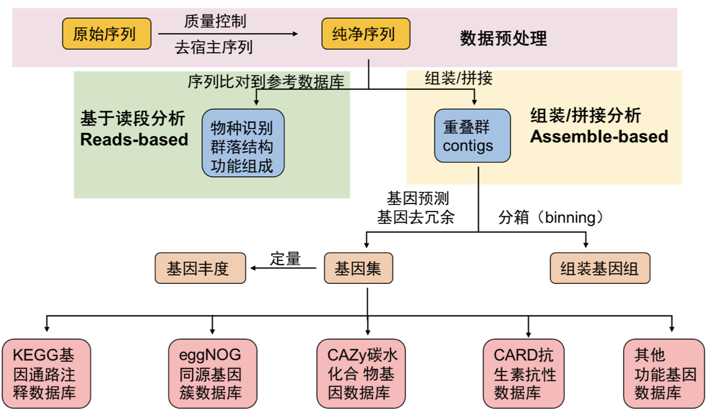
The analysis of metagenomic data typically involves the following steps:
- DNA Extraction and Library Preparation:
- DNA is extracted from environmental samples, followed by library preparation to amplify the genetic material for sequencing.
- High-Throughput Sequencing:
- The amplified DNA is subjected to high-throughput sequencing techniques to generate raw sequence data.
- Data Cleaning and Assembly:
- Raw sequence data undergo quality control procedures to remove low-quality and redundant sequences. The remaining sequences are assembled into longer contiguous sequences (contigs).
- Gene Annotation:
- Genes within the contigs are annotated to assign functional information to them, providing insights into the genetic content of the metagenome.
- Data Analysis:
- Analyzing microbial diversity, community structure, functional features, etc., often involves further analysis after obtaining abundance tables for species or functional features.
- MAGs (Metagenome-Assembled Genomes) Binning and Evolutionary Dynamics:
- Additional analyses may include the binning of MAGs to reconstruct individual genomes from metagenomic data and exploring evolutionary dynamics.
This represents a common workflow (Figure 11.1) that can be adapted and modified based on the specific requirements and objectives of each project. Depending on the project, additional steps or modifications may be necessary to address specific research questions or challenges.
In most cases, upstream data analysis needs to be performed on a cluster, typically running on a Linux system. pctax provides convenient functionalities to adapt to your data and generate corresponding Slurm scripts for execution in a cluster environment. This allows you to easily integrate pctax into your data processing pipeline and leverage the computational resources of the cluster to expedite the data analysis process.
#!/bin/bash
#SBATCH --job-name=fastp
#SBATCH --output=~/test_project/log/%x_%A_%a.out
#SBATCH --error=~/test_project/log/%x_%A_%a.err
#SBATCH --array=1
#SBATCH --partition=cpu
#SBATCH --nodes=1
#SBATCH --tasks-per-node=1
#SBATCH --cpus-per-task=1
#SBATCH --mem-per-cpu=2G
samplelist=~/test_project/samplelist

echo start: `date +"%Y-%m-%d %T"`
start=`date +%s`

####################
echo "SLURM_ARRAY_TASK_ID: " $SLURM_ARRAY_TASK_ID
START=$SLURM_ARRAY_TASK_ID

NUMLINES=40 #how many sample in one array

STOP=$((SLURM_ARRAY_TASK_ID*NUMLINES))
START="$(($STOP - $(($NUMLINES - 1))))"

#set the min and max
if [ $START -lt 1 ]
then
  START=1
fi
if [ $STOP -gt 40 ]
then
  STOP=40
fi

echo "START=$START"
echo "STOP=$STOP"

####################
for (( N = $START; N <= $STOP; N++ ))
do
  sample=$(head -n "$N" $samplelist | tail -n 1)
  echo $sample
  mkdir -p data/fastp
  ~/miniconda3/envs/waste/bin/fastp -w 8 -i data/rawdata/${sample}_f1.fastq.gz -o data/fastp/${sample}_1.fq.gz \
    -I data/rawdata/${sample}_r2.fastq.gz -O data/fastp/${sample}_2.fq.gz -j data/fastp/${i}.json
done

##############
echo end: `date +"%Y-%m-%d %T"`
end=`date +%s`
echo TIME:`expr $end - $start`s
There are many built-in steps in the micro_sbatch: c(“fastp”,“rm_human”,“kraken”,“kraken2”,“megahit”,“megahit2”,“prodigal”,“cluster”,“seq_stat”,“salmon-index”,“salmon-quant”,“salmon-merge”,“eggnog”,“cazy”,“rgi”,“vfdb”,“summary”).
flowchart TD
  A[rawdata] -- fastp, rm_human --> B[cleandata]
  B[cleandata] -- kraken2 --> C[taxa abundance]:::abundance
  B -- megahit --> D[contigs]
  D[contigs] -- prodigal --> E[genes]
  E -- cluster --> F[Non-redundant genes]
  F -- salmon-index --> G[NR index]
  G[NR index] & B --salmon-quant, salmon-merge -->H[gene abundance]:::abundance
  F -- eggnog --> I[eggnog result]:::result
  F -- cazy --> J[cazy result]:::result
  F -- rgi --> K[rgi result]:::result
  F -- vfdb --> L[vfdb result]:::result
  I --> M[annotation result]
  J --> M
  K --> M
  L --> M
  M & H -- summary --> N[annotation abundance]:::abundance
classDef result fill:#f9f,stroke:#333,stroke-width:4px
classDef abundance fill:#6EC3E0,stroke:#333,stroke-width:3px
micro_sbatch
11.2 fastp
Fastp is a versatile tool commonly used for preprocessing high-throughput sequencing data, particularly for quality control and adapter trimming. It offers a range of functionalities, including read filtering, adapter removal, quality trimming, and error correction, all in a fast and memory-efficient manner.
One notable feature of Fastp is its ability to generate JSON-formatted reports summarizing various metrics related to read quality and processing steps. These reports provide detailed statistics about the input data, such as the number of reads processed, quality distribution, adapter content, and trimming statistics. Additionally, the JSON output includes information about the filtering and processing steps applied to the data, facilitating thorough quality assessment and downstream analysis.
We can use pre_fastp to prepare the json files from fastp:
pre_fastp("my_reads.json")