| Method | Description |
|---|---|
| cpm | Counts per million |
| minmax | linear transfer to (min, max) |
| acpm | Counts per million, then asinh transfer |
| log1 | $log(n+1)$ transformat |
| total | divide by total |
| max | divide by maximum |
| frequency | divide by total and multiply by the number of non-zero items, so that the average of non-zero entries is one. |
| normalize | make margin sum of squares equal to one |
| range | standardize values into range (0,1) (same to minmax(0,1)). If all values are constant, they will be transformed to 0. |
| rank | rank replaces abundance values by their increasing ranks leaving zeros unchanged. |
| rrank | rrank is similar but uses relative ranks with maximum 1. |
| pa | scale x to presence/absence scale (0/1). |
| standardize | scale x to zero mean and unit variance. |
| hellinger | square root of method = "total" |
| log | logarithmic transformation as suggested by Anderson et al. (2006): $log_b(x)+1$ for x>0, where b is the base of the logarithm; zeros are left as zeros. |
| alr | Additive log ratio ('alr') transformation (Aitchison 1986) reduces data skewness and compositionality bias. |
| clr | centered log ratio ('clr') transformation proposed by Aitchison (1986) reduces data skewness and compositionality bias. |
| rclr | robust clr ('rclr') is similar to regular clr (see above) but allows data that contains zeroes. |
3 Explore composition
3.1 Pre-processing
The trans() function contains many normalization methods, suitable for pre-processing of different omics, some refer to vegan::decostand().
trans(otutab, method = "log1") %>% head()| NS1 | NS2 | NS3 | NS4 | NS5 | NS6 | WS1 | WS2 | WS3 | WS4 | WS5 | WS6 | CS1 | CS2 | CS3 | CS4 | CS5 | CS6 | |
|---|---|---|---|---|---|---|---|---|---|---|---|---|---|---|---|---|---|---|
| s__un_f__Thermomonosporaceae | 6.996682 | 7.560601 | 6.698268 | 7.211557 | 6.970730 | 6.976348 | 7.133296 | 7.376508 | 7.193686 | 6.848005 | 7.118016 | 6.919684 | 7.746733 | 7.831617 | 7.444249 | 7.588830 | 7.266827 | 7.331715 |
| s__Pelomonas_puraquae | 7.582229 | 7.118826 | 7.767687 | 7.712891 | 7.973844 | 7.512071 | 6.469250 | 6.206576 | 7.115582 | 7.158514 | 6.860664 | 6.455199 | 7.174724 | 7.324490 | 6.739337 | 7.029088 | 7.302496 | 7.069023 |
| s__Rhizobacter_bergeniae | 6.378426 | 6.129050 | 6.791221 | 6.804614 | 7.112327 | 6.749931 | 6.405228 | 6.154858 | 6.976348 | 6.936343 | 6.741701 | 6.508769 | 6.937314 | 7.497207 | 6.910751 | 7.090910 | 7.085902 | 6.637258 |
| s__Flavobacterium_terrae | 5.501258 | 5.459586 | 7.501634 | 6.513230 | 7.276556 | 6.198479 | 5.765191 | 7.563720 | 7.309212 | 6.903747 | 6.359574 | 5.886104 | 6.985642 | 7.105786 | 6.626718 | 6.049734 | 6.940222 | 7.253470 |
| s__un_g__Rhizobacter | 7.267525 | 6.023448 | 6.280396 | 6.633318 | 7.162397 | 6.228511 | 6.222576 | 6.381816 | 6.100319 | 6.431331 | 6.489205 | 6.063785 | 7.032624 | 7.277939 | 6.311735 | 6.369901 | 7.008505 | 6.806829 |
| s__un_o__Burkholderiales | 6.787845 | 6.527958 | 6.715383 | 6.816736 | 7.315218 | 6.937314 | 5.463832 | 5.533390 | 5.886104 | 5.945421 | 5.961005 | 5.863631 | 6.313548 | 6.293419 | 6.169611 | 6.327937 | 6.242223 | 6.208590 |
rm_low(), guolv() and hebing() functions can help filter or aggregate the omics data.
3.2 Stackplot
# sum the abundance to Phylum level
hebing(otutab, taxonomy$Phylum, margin = 1, act = "sum") -> phylum
stackplot(phylum, metadata, group = "Group", topN = 10) +
  scale_fill_manual(values = get_cols(10))
stackplot(phylum, metadata,
  group = "Group", style = "sample",
  group_order = TRUE, flow = TRUE, relative = FALSE
) +
  scale_fill_manual(values = get_cols(10))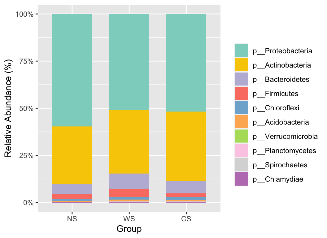
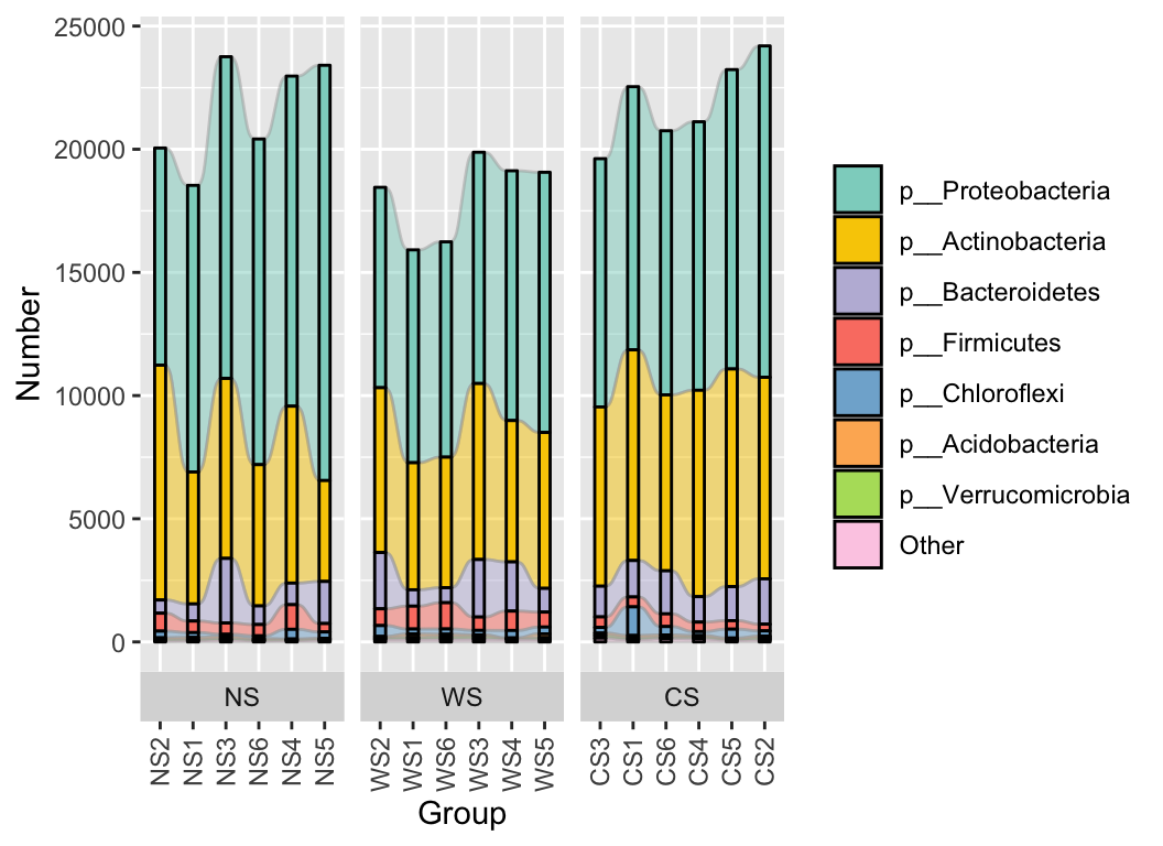
The stackplot function offers a wide range of parameters to facilitate the adjustment of the final graphical output. For further details and examples on drawing bar plots and their transformations in R, please refer to R Draw the bar plot and its transformation.
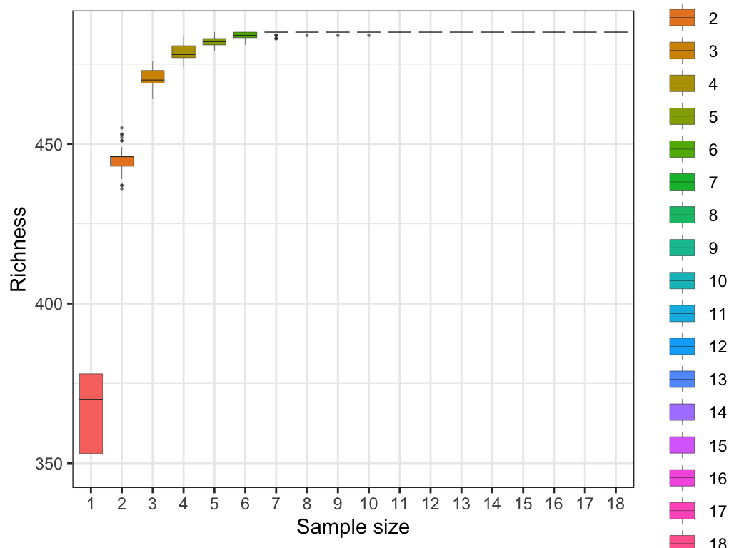
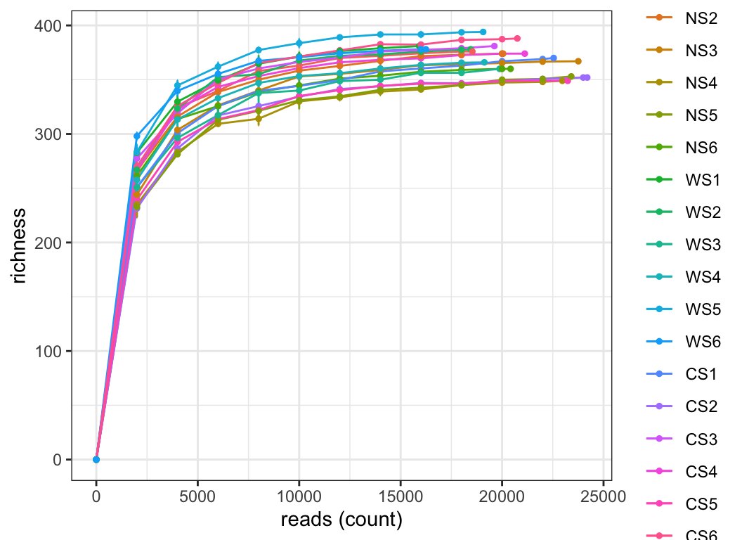
3.3 Rarefaction
Rarefaction is a method used to assess the relationship between sample community data sampling effort and species richness within the sample. Commonly used in ecology, it evaluates whether the observed species diversity saturates given a certain number of samples or sequences, and whether additional sampling is needed to fully capture species richness within the sample.
For sample data, Rarefaction curves display the number of observed species at different levels of sampling effort (or sequence numbers). By plotting Rarefaction curves, one can assess how species diversity changes with varying sampling depths and determine if saturation has been reached.
For species data, Rarefaction curves display the number of observed samples at different levels of sampling effort (or sequence numbers). Through this method, one can evaluate how sample numbers change with different sampling depths and determine if additional samples are necessary to fully capture species richness.
3.4 Phylogenetic tree
ann_tree(taxonomy, otutab) -> tree
easy_tree(tree, add_abundance = FALSE)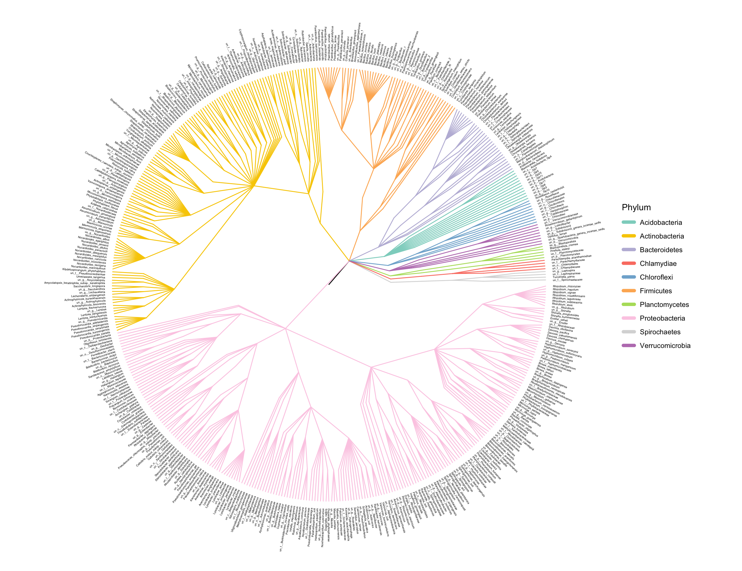
easy_tree(tree, add_tiplab = FALSE) -> p
some_tax <- table(taxonomy$Phylum) %>%
  sort(decreasing = TRUE) %>%
  head(5) %>%
  names()
add_strip(p, some_tax)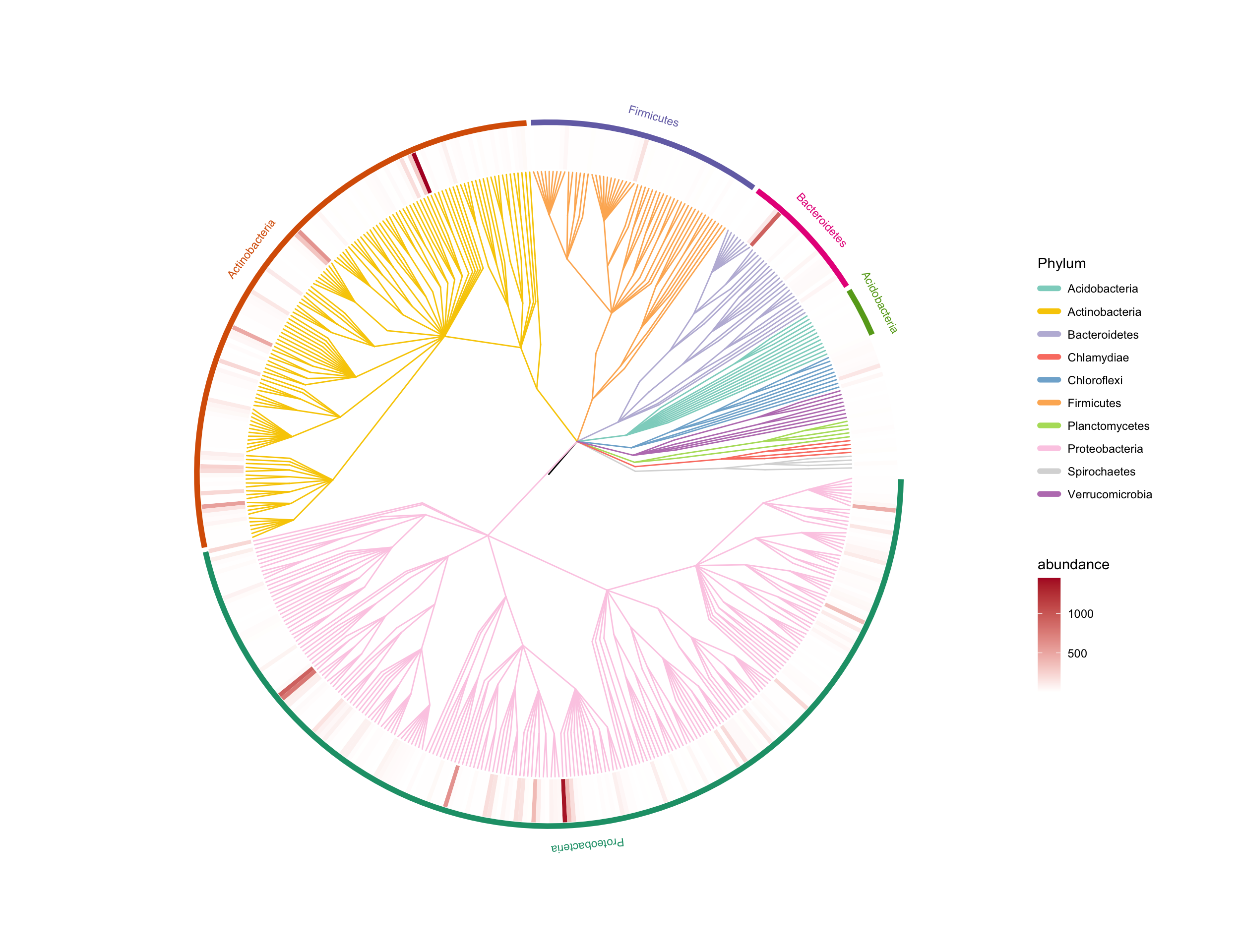
You can refer to Basic phylogenetic tree and Advanced phylogenetic tree to plot the phylogenetic tree using ggtree.
In addition, you can also choose to use online platforms like iPhylo and iTOL for interactive plotting.
iPhylo is a free online platform for generating, annotating, and visualizing phylogenetic trees. It allows you to plot various tree diagrams for species, compounds, and other hierarchical structures and conveniently add complex annotation information.
iPhylo Website: https://iphylo.net
For more information, you can check out our Online Guide Book.
sangji_plot(tree, width = 900, height = 700)sunburst(tree)3.5 Rtaxonkit
Taxonkit is a Practical and Efficient NCBI Taxonomy Toolkit (1).
We recommend you download this excellent software to help next analysis. Or you can use Taxonkit in R by pctax interface as followed:
# 1. This function help you install suitable version taxonkit
install_taxonkit()
# taxonkit has been successfully installed!

# 2. Then download the NCBI taxonomy database.
download_taxonkit_dataset()
# Taxonkit files downloaded and copied successfully.

# 3. Check whether taxonkit is ready
check_taxonkit()
# ==============Taxonkit is available if there is help message above==============
# =========================Taxonkit dataset is available!=========================
Then you can use taxonkit in R just like in terminal.
?taxonkit_lineage

# taxonkit_list
# taxonkit_reformat
# taxonkit_name2taxid
# taxonkit_filter
# taxonkit_lca
lineage <- taxonkit_lineage("9606\n63221", show_name = TRUE, show_rank = TRUE, text = T)
lineage[1] "9606\tcellular organisms;Eukaryota;Opisthokonta;Metazoa;Eumetazoa;Bilateria;Deuterostomia;Chordata;Craniata;Vertebrata;Gnathostomata;Teleostomi;Euteleostomi;Sarcopterygii;Dipnotetrapodomorpha;Tetrapoda;Amniota;Mammalia;Theria;Eutheria;Boreoeutheria;Euarchontoglires;Primates;Haplorrhini;Simiiformes;Catarrhini;Hominoidea;Hominidae;Homininae;Homo;Homo sapiens\tHomo sapiens\tspecies"
[2] "63221\tcellular organisms;Eukaryota;Opisthokonta;Metazoa;Eumetazoa;Bilateria;Deuterostomia;Chordata;Craniata;Vertebrata;Gnathostomata;Teleostomi;Euteleostomi;Sarcopterygii;Dipnotetrapodomorpha;Tetrapoda;Amniota;Mammalia;Theria;Eutheria;Boreoeutheria;Euarchontoglires;Primates;Haplorrhini;Simiiformes;Catarrhini;Hominoidea;Hominidae;Homininae;Homo;Homo sapiens;Homo sapiens neanderthalensis\tHomo sapiens neanderthalensis\tsubspecies"