6 Clustering analysis
Cluster analysis, also known as clustering, is a powerful technique used to identify patterns within abundance tables or datasets. It works by grouping data points into clusters based on their similarities or dissimilarities. In the context of abundance tables, cluster analysis can help uncover the main patterns or structures present in the data, such as groups of samples with similar microbial compositions.
By applying clustering algorithms to abundance tables, researchers can identify distinct clusters of samples that share similar abundance profiles. These clusters may represent different microbial communities or community states within the dataset. Clustering analysis enables researchers to explore the underlying structure of the data, identify potential outliers or anomalies, and gain insights into the overall composition and organization of microbial communities.
6.1 Fuzzy C-means
Fuzzy C-means (FCM) clustering is a popular algorithm used for partitioning data points into clusters in a dataset. Unlike traditional K-means clustering, FCM allows each data point to belong to multiple clusters with varying degrees of membership, making it a soft clustering algorithm.
In FCM, each data point is assigned a membership value for each cluster, representing the degree to which it belongs to that cluster. These membership values are determined based on minimizing an objective function, typically the fuzzy objective function, which quantifies the similarity between data points and cluster centroids while considering the fuzziness of cluster membership.
The algorithm iteratively updates cluster centroids and membership values until convergence is achieved. FCM is widely used in various fields, including pattern recognition, image segmentation, and bioinformatics, for its ability to identify complex patterns and accommodate uncertainty in data clustering.
library(ReporterScore)
pcutils::hebing(otutab, metadata$Group) -> otu_group
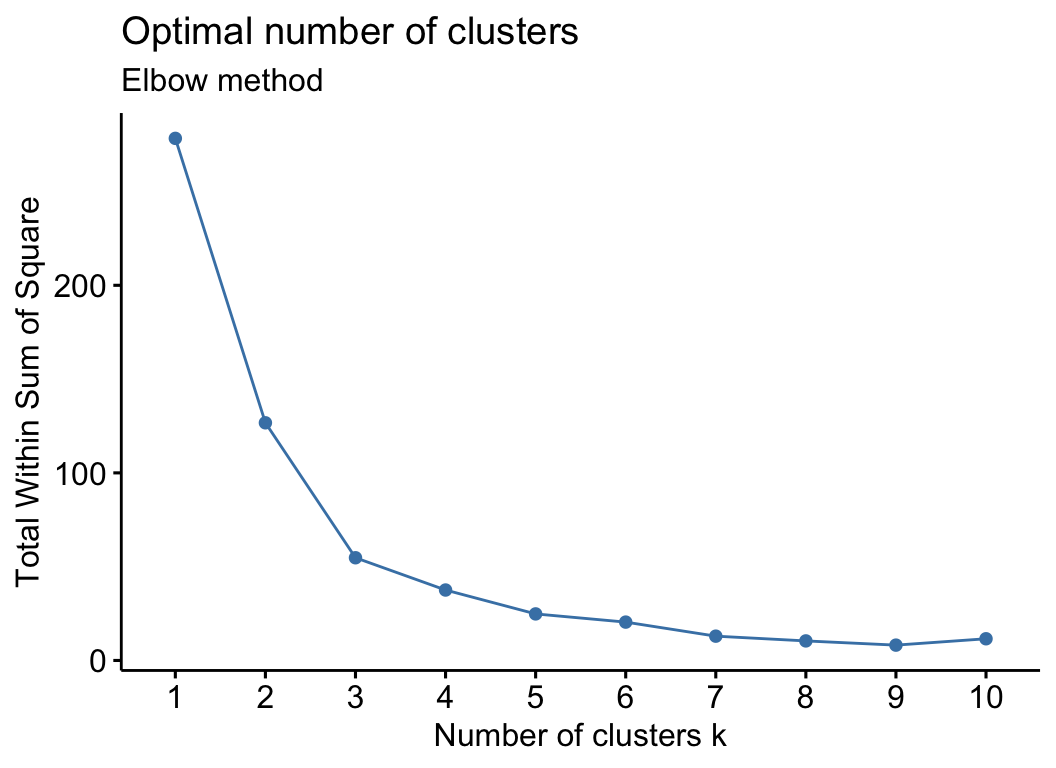
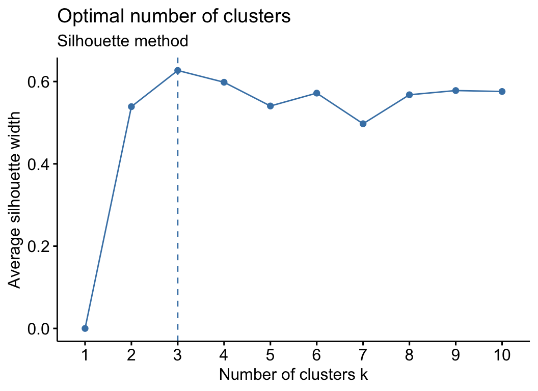
cm_test_k(otu_group, filter_var = 0.7)
## $cp1
##
## $cp2
##
## $cp3
## NULL
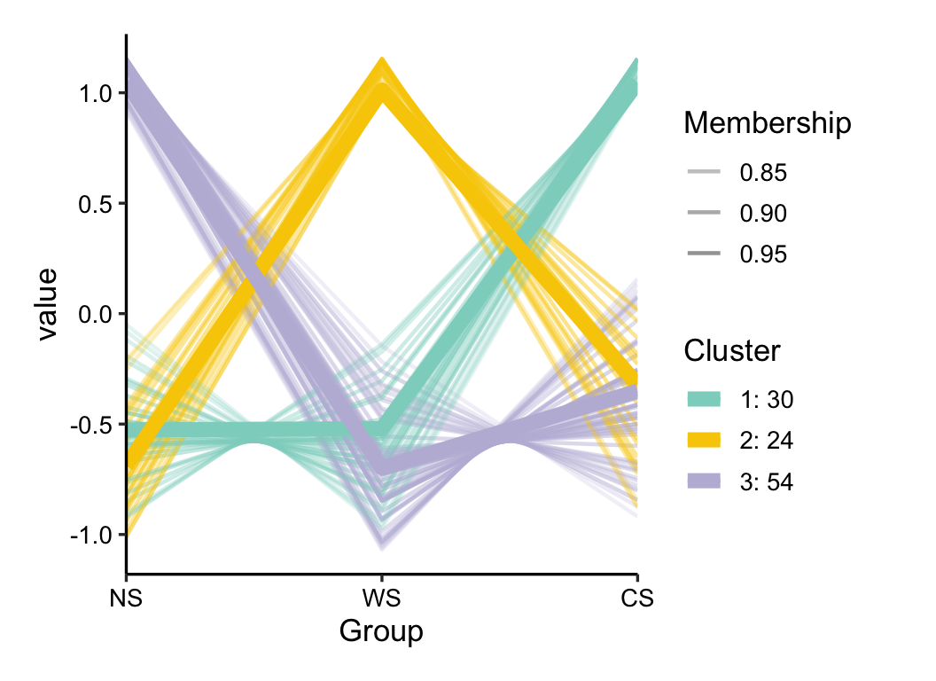
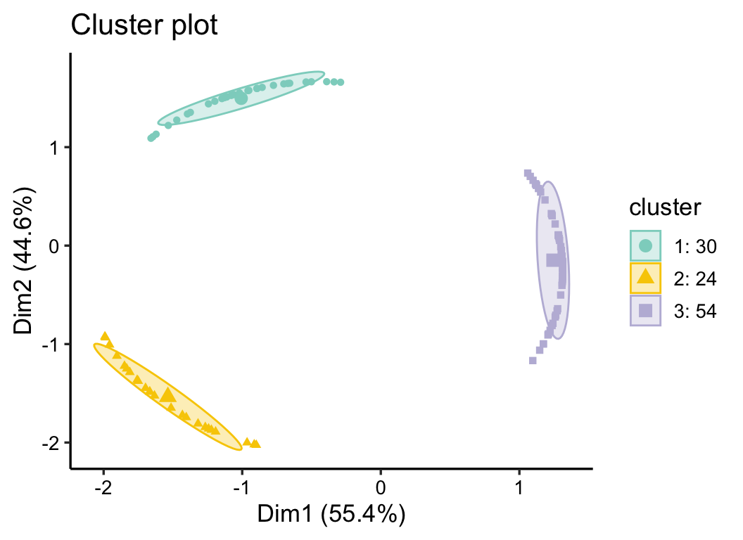
cm_res <- c_means(otu_group, k_num = 3, filter_var = 0.7)
plot(cm_res, 0.8)
plot(cm_res, 0.8, mode = 2)