Chapter 3 t-test & ANOVA
3.1 Warm-up activity for fun - can you replace my name with yours using the following functions?
paste("Today is", date())## [1] "Today is Mon Aug 22 12:20:23 2022"name <- "Jimmy"
state <- "California"
print(name) #this syntax is more intuitive## [1] "Jimmy"paste(name, "lives in", state)## [1] "Jimmy lives in California"3.1.1 If you are a first-time R user, please follow the following tip to set up your working directory:
You need forward slashes in the path, not backslashes (which caught me out when I started using R). So perhaps you should try: data1<- read.table(file=“C:/Users/yourusername/Desktop/grapeJuice.csv”,header=TRUE). Please make sure to replace ‘yourusername’ in the above path with your real username. For instanc, my current user name is zxu3.
Read the tips below if you do not know your username: https://regroove.ca/oh365eh/2015/04/12/how-to-find-your-user-name-on-your-pc/
3.1.2 Research design - Review our Research Design tutorial
H0- Null hypotheses use as basis for argument but has not yet proven, no difference prediction (all equal).
H1 - Alternative hypotheses statement set-up to establish like new effect compared to existing (e.g new drug is better than the existing standard products).
3.2 Introduction
Which type of in-store advertisement is more effective? To answer this question, the marketing team decided to place two types of ads in a pilot store for testing using two themes of juices: one theme is natural production of the juice, and the other theme is family health caring. The goal of this experiment is to see if they can place the better one into all of the stores after the pilot period.
3.2.1 Research design issues
In this study, we analyze the effectiveness of ads on sales using Welch’s independent sample t-test. Here independent means that points (i.e., (i.e., customers in this case)) do not match up with each other.
Alternatively, for instance, we might perform a paired sample t test in which we could test if a ‘before’ (let consumers be exposed to natural themes) and ‘after’(let consumers be exposed to family themes) condition will affect the sales of each store.
3.2.2 Variable Description
Sales: Total unit sales of the grape juice in one week in a store Price: Average unit price of the grape juice in the week ad_type: The in-store advertisement type to promote the grape juice.ad_type = 0, the theme of the ad is natural production of the juice ad_type = 1, the theme of the ad is family health caring price_apple: Average unit price of the apple juice in the same store in the week price_cookies: Average unit price of the cookies in the same store in the week
3.2.3 Step 1:
Please write a null hypothesis and an alternative hypothesis using the template hypotheses available in the research design module.
3.2.4 Step 2:
Please make your conclusions based on the results in descriptive analysis 3. What is your conclusion?
We performed a normality test in Step - normality check 1. What is your conclusion?
Hint: read the third reference article.
3.2.5 Step 3: Perform a t-test using Excel or R
3.2.6 Step 3.1 Perform a t-test using Excel
In this step, you will be performing a t-test using Excel. Once you get the result, please attach your output Spreadsheet in the discussion forum.
Reference: Excel - Independent samples Welch t test (via data analysis) https://www.youtube.com/watch?v=sHqCrK_FMyY
3.2.7 Step 3.2 (Preparation & debugging)
In this step, you will be performing the t-test again using R and R studio. The goal is to help you document your analysis for future reference.
Please try to perform the analysis using R and Rpubs before the class on Thursday and post your final bugs and errors (or the final URL of your Rpubs page) to receive participation credits toward your final Engagement grade.
Note: For details about “Preparation & debugging,” please read the section “Preparation & debugging” in the Syllabus or the Syllabus page of LMS.
The “Preparation & debugging” can be frustrating for statistics majors sometimes. Do not be panic!!! I hope you could recognize the challenge as an opportunity for you to build a stronger sense of self. You may find the following testimony by Thomas Mock helpful. Please also try to watch the YouTube video “R Programming Tutorial - Learn the Basics of Statistical Computing” to get familiar with the R basics.
“Within the first month of the course I actually reverted back to doing things in Systat with a GUI as I was so frustrated with not knowing what I was doing in R.”
References:
My R Journey: Thomas Mock https://rfortherestofus.com/2019/09/my-r-journey-thomas-mock/
R Programming Tutorial - Learn the Basics of Statistical Computing: https://www.youtube.com/watch?v=_V8eKsto3Ug
3.2.8 Step 4: Wrap-up - interpret the results
We performed a Welch’s t test in the step 3. What is your conclusion?
Hint: read the first three reference articles. Make sure to cite.
3.2.9 Descriptive Analysis 1:
library(readr)
data <- read_csv("https://raw.githubusercontent.com/utjimmyx/ttest/master/grapeJuice.csv")
## New names:
## Rows: 30 Columns: 6
## -- Column specification
## -------------------------------------------------------- Delimiter: "," dbl
## (6): ...1, Sales, price, ad_type, price_apple, price_cookies
## i Use `spec()` to retrieve the full column specification for this data. i
## Specify the column types or set `show_col_types = FALSE` to quiet this message.
## * `` -> `...1`head(data) #view the first 6 lines| ...1 | Sales | price | ad_type | price_apple | price_cookies |
|---|---|---|---|---|---|
| 1 | 222 | 9.83 | 0 | 7.36 | 8.8 |
| 2 | 201 | 9.72 | 1 | 7.43 | 9.62 |
| 3 | 247 | 10.2 | 1 | 7.66 | 8.9 |
| 4 | 169 | 10 | 0 | 7.57 | 10.3 |
| 5 | 317 | 8.38 | 1 | 7.33 | 9.54 |
| 6 | 227 | 9.74 | 0 | 7.51 | 9.49 |
#perform some basic descriptive analysis
summary(data)
## ...1 Sales price ad_type price_apple
## Min. : 1.00 Min. :131.0 Min. : 8.200 Min. :0.0 Min. :7.300
## 1st Qu.: 8.25 1st Qu.:182.5 1st Qu.: 9.585 1st Qu.:0.0 1st Qu.:7.438
## Median :15.50 Median :204.5 Median : 9.855 Median :0.5 Median :7.580
## Mean :15.50 Mean :216.7 Mean : 9.738 Mean :0.5 Mean :7.659
## 3rd Qu.:22.75 3rd Qu.:244.2 3rd Qu.:10.268 3rd Qu.:1.0 3rd Qu.:7.805
## Max. :30.00 Max. :335.0 Max. :10.490 Max. :1.0 Max. :8.290
## price_cookies
## Min. : 8.790
## 1st Qu.: 9.190
## Median : 9.515
## Mean : 9.622
## 3rd Qu.:10.140
## Max. :10.5803.2.10 Descriptive Analysis 2:
#set the 1 by 2 layout plot window
par(mfrow=c(1,2))
#Check if there are outliers using a boxplot
#Let's perform boxplots in two different ways
boxplot(data$Sales,main="Boxplot for sales data", ylab="Sales")
boxplot(data$Sales,main="Boxplot for sales data", horizontal = TRUE, xlab="Sales")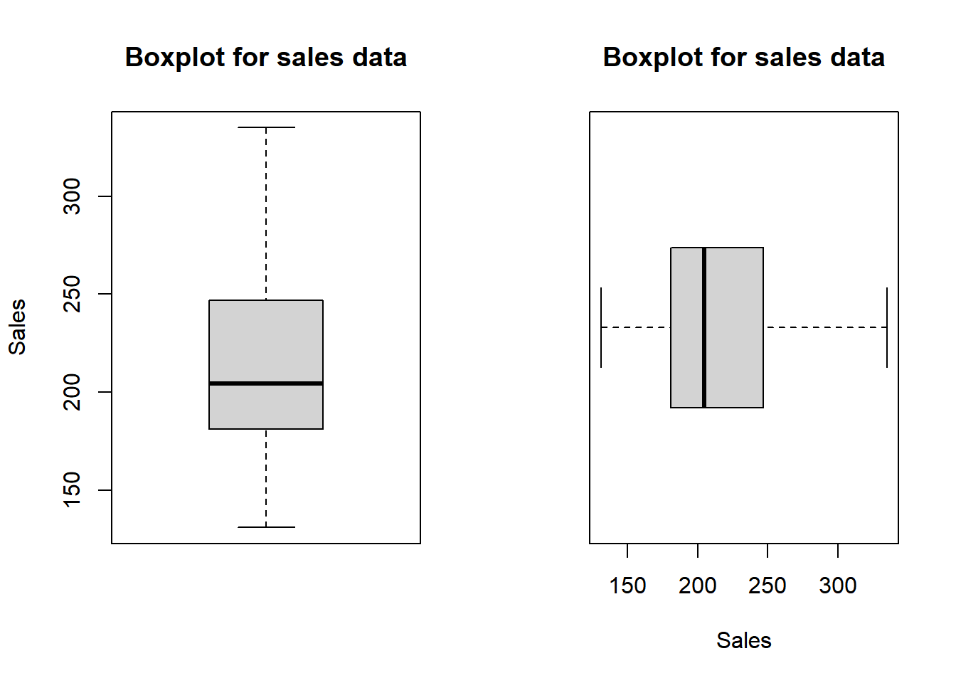
#Let's perform a histogram analysis
hist(data$Sales,main='histogram plot for sales data',xlab='sales_grape',prob=T)
lines(density(data$Sales),lty='dashed',lwd=2.5, col='blue')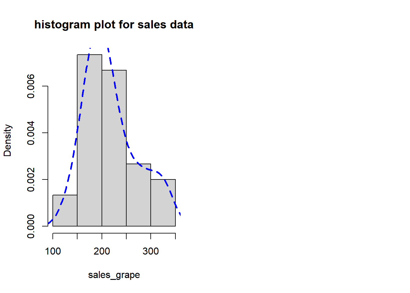
It seems that there is no outlieer and the distribution of the data is roughly normal.
3.2.11 Descriptive analysis 3 - Compare the mean of sales with the two different ad types
#divide the dataset into two sub dataset by ad_type
sales_ad_nature = subset(data,ad_type==0)
sales_ad_family = subset(data,ad_type==1)

#calculate the mean of sales with different ad_type
mean(sales_ad_nature$Sales)
## [1] 186.6667mean(sales_ad_family$Sales)## [1] 246.66673.3 Assumption check 1
The assumptions of t-tests assumes the observations are normally distributed and independent.
#set the 1 by 2 layout plot window
par(mfrow = c(1,2))

# Explore the distribution of the data using histogram
hist(sales_ad_nature$Sales,main="",xlab="sales with nature theme ad",prob=T)
lines(density(sales_ad_nature$Sales),lty="dashed",lwd=2.5,col="red")

hist(sales_ad_family$Sales,main="",xlab="sales with family theme ad",prob=T)
lines(density(sales_ad_family$Sales),lty="dashed",lwd=2.5,col="red")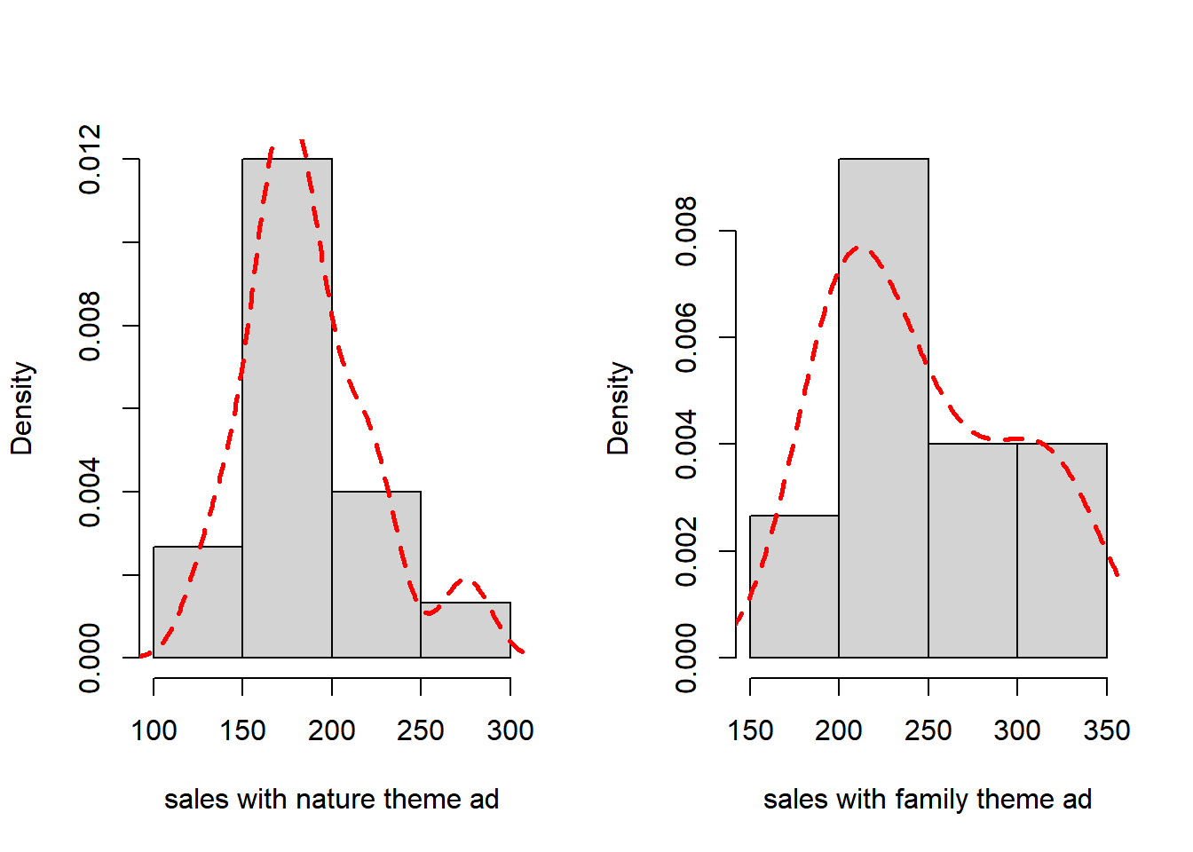
#set the 1 by 2 layout plot window
par(mfrow = c(1,2))

# boxplot to check if there are outliers in each group
boxplot(sales_ad_family$Sales,horizontal = TRUE, xlab="sales with family theme ad")
boxplot(sales_ad_nature$Sales,horizontal = TRUE, xlab="sales with nature theme ad")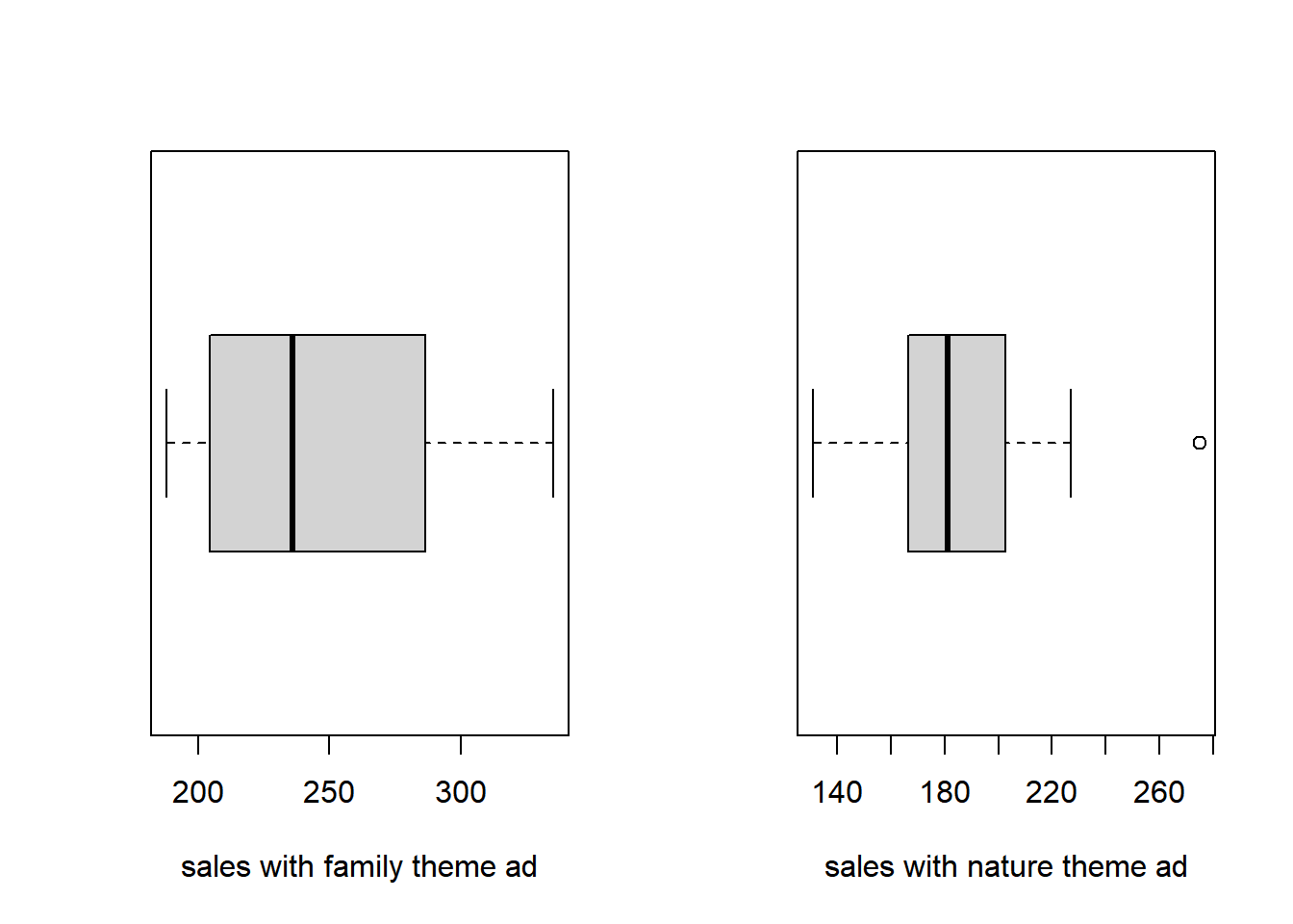
3.3.1 Let’s build a more elegant boxplot with ggplot (the most elegant and aesthetically pleasing graphics framework available)
3.3.2 First we convert the variable ad_type from a numeric to a factor variable
data$ad_type <- as.factor(data$ad_type)
head(data)| ...1 | Sales | price | ad_type | price_apple | price_cookies |
|---|---|---|---|---|---|
| 1 | 222 | 9.83 | 0 | 7.36 | 8.8 |
| 2 | 201 | 9.72 | 1 | 7.43 | 9.62 |
| 3 | 247 | 10.2 | 1 | 7.66 | 8.9 |
| 4 | 169 | 10 | 0 | 7.57 | 10.3 |
| 5 | 317 | 8.38 | 1 | 7.33 | 9.54 |
| 6 | 227 | 9.74 | 0 | 7.51 | 9.49 |
# Import the ggplot library
library(ggplot2)
##
## Attaching package: 'ggplot2'## The following object is masked from 'package:huxtable':
##
## theme_grey# Wait for the magic to happen
ggplot(data, aes(x=ad_type, y=Sales, fill=ad_type))+
geom_boxplot(outlier.shape = NA, alpha=.5) +
geom_jitter(width=.1, size=1) +
theme_classic() +
scale_fill_manual(values=c("lightseagreen","darkseagreen"))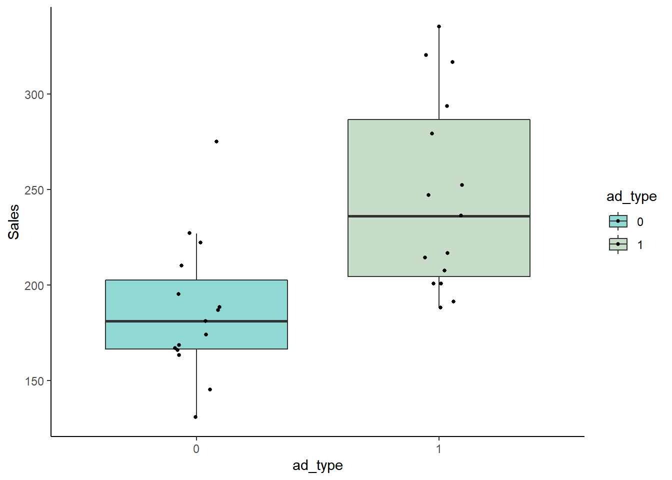
3.4 Assumption check 2
In this step, we perform a Shapiro test to see if our data is from a normaly distributed population.
shapiro.test(sales_ad_nature$Sales)##
## Shapiro-Wilk normality test
##
## data: sales_ad_nature$Sales
## W = 0.94255, p-value = 0.4155shapiro.test(sales_ad_family$Sales)##
## Shapiro-Wilk normality test
##
## data: sales_ad_family$Sales
## W = 0.89743, p-value = 0.086953.5 t-test
Performing a t-test with which has two categories (e.g., Controlled and Treated) helps us understand if there are differences in the population means between the two groups.
“mu=0” refers to the null hypothesis that the difference between Control and Treated is 0, and hence they are similar. alt=“two.sided” refers to the a two sided t test. conf=0.95 is the confidence interval.
t.test(Sales ~ ad_type, data)##
## Welch Two Sample t-test
##
## data: Sales by ad_type
## t = -3.7515, df = 25.257, p-value = 0.0009233
## alternative hypothesis: true difference in means between group 0 and group 1 is not equal to 0
## 95 percent confidence interval:
## -92.92234 -27.07766
## sample estimates:
## mean in group 0 mean in group 1
## 186.6667 246.6667library(pander)##
## Attaching package: 'pander'## The following object is masked from 'package:huxtable':
##
## wrappanderOptions('round',4)
panderOptions('digits',7)
panderOptions('keep.trailing.zeros',TRUE)
panderOptions("table.split.table", Inf)
pander(t.test(sales_ad_nature$Sales,sales_ad_family$Sales))| Test statistic | df | P value | Alternative hypothesis | mean of x | mean of y |
|---|---|---|---|---|---|
| -3.7515 | 25.2571 | 9e-04 * * * | two.sided | 186.6667 | 246.6667 |
3.5.1 Google & StackOverflow are definitely the top go-to choices for developers and programmers at any level
For R-related questions, use https://stackoverflow.com/questions/tagged/r
For statistics related questions, use https://stats.stackexchange.com.
Data Science Specialization at John Hopkins University, https://www.coursera.org/specializations/jhu-data-science
3.5.2 Reference
Two Independent Samples Unequal Variance (Welch’s Test) https://sites.nicholas.duke.edu/statsreview/means/welch/
ANOVA, t-tests and regression: different ways of showing the same thing http://deevybee.blogspot.com/2017/11/anova-t-tests-and-regression-different.html
The Independent Samples t-test (Welch Test) https://stats.libretexts.org/Bookshelves/Applied_Statistics/Book%3A_Learning_Statistics_with_R_-_A_tutorial_for_Psychology_Students_and_other_Beginners_(Navarro)/13%3A_Comparing_Two_Means/13.04%3A_The_Independent_Samples_t-test_(Welch_Test)
https://en.wikipedia.org/wiki/Shapiro%E2%80%93Wilk_test
My R Journey: Thomas Mock https://rfortherestofus.com/2019/09/my-r-journey-thomas-mock/
R Programming Tutorial - Learn the Basics of Statistical Computing: https://www.youtube.com/watch?v=_V8eKsto3Ug
Pander Library 1. https://www.r-project.org/nosvn/pandoc/pander.html
Generating-tables-using-pander-knitr.https://r-norberg.blogspot.com/2013/06/generating-tables-using-pander-knitr.html