Chapter 4 Basic regression analysis

################################################################################
##      Predictive Modeling for Los Angeles Dodgers Promotion and Attendance (R)
##        by Dr. Jimmy (Zhenning) Xu, 
##        follow me on Twitter https://twitter.com/MKTJimmyxu
################################################################################

4.1 What is a regression analysis?

The following video is about the statistics about the aircrafts during WW2. Military command initially proposed reinforcing the most damaged areas. At first sight, this seems to make sense. But think a little harder and you realize it doesn’t.

Battle of Britain Statistics | Allied and Axis Losses

https://www.youtube.com/watch?v=O3AsxBQzkmI

The commanders were focusing on the planes that came back, not on those that didn’t. The areas that needed protection were not the ones damaged in returning planes. They were the ones that were not damaged, because those provided a clue on the hits that shot down planes.

This is a classic example of survival bias, one of the most common problems when people try to make sense of data. People tend to ignore the process by which data were selected. It’s everywhere in business.

The bias stems from the general tendency for people to focus on what is known and not sufficiently on what is not known.

(Content from our Rules for Effective Decision Making program: https://lnkd.in/emv5EpF, with Bart De Langhe.)

Regression is a technique used to analyze the relationship between a dependent (criterion) variable and one or more independent (predictor) variables.

We need an interval dependent variable and either interval or binary independent variables.

Regression equation: Y = bo + b1x1 + b2x2 + …

How Are Correlation and Regression Related?

The square of the correlation is R2 - gives the explained variance of the dependent variable by the independent variable(s)

- called the coefficient of determination (R2)

4.2 Example Regression equation:

     Y = 56 + 4.63*x1 + 9.87*x2

Food Sales = bo + advert. + coupons

Q1: How to interpret the coefficient for X1 (advert.)? Please share your answer with us.

Q2: From the previous regression equation, let’s say we get an R2 of .54.

How to interpret R square? Please share your answer with us.

Q3: What are other questions that could be answered using this regression model? Please refer to Page 75 of the following book (free access):

https://faculty.marshall.usc.edu/gareth-james/ISL/ISLR%20Seventh%20Printing.pdf

Important Tips: You can find the answers to the discussion questions in Week 2 - Research Design (Lab 1: https://rpubs.com/utjimmyx/researchdesign) from page 59 to page 61.

4.3 Real world examples

Assume that you work for the local economic bureau, which of the following variables would you use to predict female life expectancy? 1. Infant Mortality 4. GDP 2. Fertility 5. Birth-to-death ratio 3. urban population 6. population increase

Assume that you work for the Hass Avocado Association, which variable would you use to predict avocado sales?

Assume that you work for the national beer Association, which variable would you use to predict beer sales?

Assume that you work for the national beer association, which variable would you use to predict beer sales? See the following two examples: https://www.kaggle.com/c/BeerSalesPrediction http://cs229.stanford.edu/proj2016/report/SchubertZylberglejd-PredictingBeerSalesInMexico-report.pdf

For more examples, please visit the 1st module in Canvas.

4.4 Introduction

It is tough to make good predictions. The numerous factors or variables, independent and dependent, involved in many sporting events contribute to the unpredictability. However, using carefully-selected variables, it is still possible to make marketing promotions more accountable.

The goal of this case study is to analyze if bobblehead promotions increase attendance at Dodgers home games. Using the fitted predictive model we can predict the attendance for the game in the forthcomming season and we can predict the attendance with or without bobblehead promotion.

The motivation of this case study is to design a predictive model, and report any interesting findings to support critical business decision making.

4.4.1 Pre-Processing

Load the required libraries and the data

setwd("C:/Users/zxu3/Documents/R/regression")

#library(car)  # Package with Special functions for linear regression
library(readr)
library(lattice)  # Graphics Package
library(ggplot2) # Graphical Package

#Create a dataframe with the Dodgers Data
#DodgersData <- read.csv("DodgersData.csv")
DodgersData <- read.csv("DodgersData.csv", fileEncoding="UTF-8-BOM", header=TRUE)

4.5 Read the data - alternative solution

I also saved the data in my GitHub site for your convenience: https://raw.githubusercontent.com/utjimmyx/regression/master/DodgersData.csv

If you still could not read data to the console, please remove the following line of syntax

DodgersData <- read.csv(“DodgersData.csv”, fileEncoding=“UTF-8-BOM”, header=TRUE)

and replace it with the following two lines of syntax for the purpose of reading the new dataset.

library(readr)

DodgersData <- read_csv(“https://raw.githubusercontent.com/utjimmyx/regression/master/DodgersData.csv”)

4.6 Data cleanup and exploratory analysis

Evaluate the Structure and Re-Level the factor variables for “Day Of Week”” and “Month”” in the right order

# Check the structure for Dorder Data
str(DodgersData)

## 'data.frame':    81 obs. of  12 variables:
##  $ month      : chr  "APR" "APR" "APR" "APR" ...
##  $ day        : int  10 11 12 13 14 15 23 24 25 27 ...
##  $ attend     : int  56000 29729 28328 31601 46549 38359 26376 44014 26345 44807 ...
##  $ day_of_week: chr  "Tuesday" "Wednesday" "Thursday" "Friday" ...
##  $ opponent   : chr  "Pirates" "Pirates" "Pirates" "Padres" ...
##  $ temp       : int  67 58 57 54 57 65 60 63 64 66 ...
##  $ skies      : chr  "Clear " "Cloudy" "Cloudy" "Cloudy" ...
##  $ day_night  : chr  "Day" "Night" "Night" "Night" ...
##  $ cap        : chr  "NO" "NO" "NO" "NO" ...
##  $ shirt      : chr  "NO" "NO" "NO" "NO" ...
##  $ fireworks  : chr  "NO" "NO" "NO" "YES" ...
##  $ bobblehead : chr  "NO" "NO" "NO" "NO" ...

head(DodgersData)

Table 4.1:
month	day	attend	day_of_week	opponent	temp	skies	day_night	cap	shirt	fireworks	bobblehead
APR	10	56000	Tuesday	Pirates	67	Clear	Day	NO	NO	NO	NO
APR	11	29729	Wednesday	Pirates	58	Cloudy	Night	NO	NO	NO	NO
APR	12	28328	Thursday	Pirates	57	Cloudy	Night	NO	NO	NO	NO
APR	13	31601	Friday	Padres	54	Cloudy	Night	NO	NO	YES	NO
APR	14	46549	Saturday	Padres	57	Cloudy	Night	NO	NO	NO	NO
APR	15	38359	Sunday	Padres	65	Clear	Day	NO	NO	NO	NO

# Evaluate the factor levels for day_of_week
# levels(DodgersData$day_of_week)

# Evaluate the factor levels for month
levels(DodgersData$month)

## NULL

# First 10 rows of the data frame
head(DodgersData, 10)

Table 4.1:
month	day	attend	day_of_week	opponent	temp	skies	day_night	cap	shirt	fireworks	bobblehead
APR	10	56000	Tuesday	Pirates	67	Clear	Day	NO	NO	NO	NO
APR	11	29729	Wednesday	Pirates	58	Cloudy	Night	NO	NO	NO	NO
APR	12	28328	Thursday	Pirates	57	Cloudy	Night	NO	NO	NO	NO
APR	13	31601	Friday	Padres	54	Cloudy	Night	NO	NO	YES	NO
APR	14	46549	Saturday	Padres	57	Cloudy	Night	NO	NO	NO	NO
APR	15	38359	Sunday	Padres	65	Clear	Day	NO	NO	NO	NO
APR	23	26376	Monday	Braves	60	Cloudy	Night	NO	NO	NO	NO
APR	24	44014	Tuesday	Braves	63	Cloudy	Night	NO	NO	NO	NO
APR	25	26345	Wednesday	Braves	64	Cloudy	Night	NO	NO	NO	NO
APR	27	44807	Friday	Nationals	66	Clear	Night	NO	NO	YES	NO

4.7 Exploratory analysis (explained)

The results show that in 2012 there were a few promotions

Cap
Shirt
Fireworks
Bobblehead

We have data from April to October for games played in the Day or Night under Clear or Cloudy Skys.

Dodger Stadium has a capacity of about 56,000. Looking at the entire (sample) data shows that the stadium filled up only twice in 2012. There were only two cap promotions, three shirt promotions - not enough data for any inferences. Fireworks and Bobblehead promotions have happened a few times.

Further more there were eleven bobble head promotions and most of then (six) being on Tuesday nights.

4.8 Evaluate Attendance by Weather

#Evaluate attendance by weather
ggplot(DodgersData, aes(x=temp, y=attend/1000, color=fireworks)) + 
        geom_point() + 
        facet_wrap(day_night~skies) + 
        ggtitle("Dodgers Attendance By Temperature By Time of Game and Skies") +
        theme(plot.title = element_text(lineheight=3, face="bold", color="black", size=10)) +
        xlab("Temperature (Degree Farenheit)") +
        ylab("Attendance (Thousands)")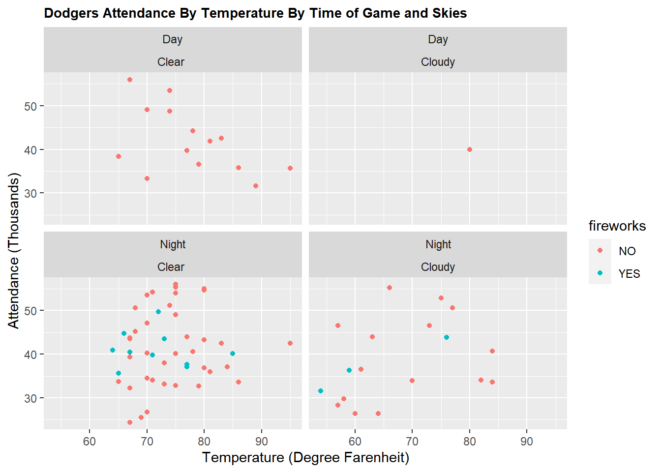

4.9 Strip Plot of Attendance by opponent or visiting team

#Strip Plot of Attendance by opponent or visiting team
ggplot(DodgersData, aes(x=attend/1000, y=opponent, color=day_night)) + 
        geom_point() + 
        ggtitle("Dodgers Attendance By Opponent") +
        theme(plot.title = element_text(lineheight=3, face="bold", color="black", size=10)) +
        xlab("Attendance (Thousands)") +
        ylab("Opponent (Visiting Team)")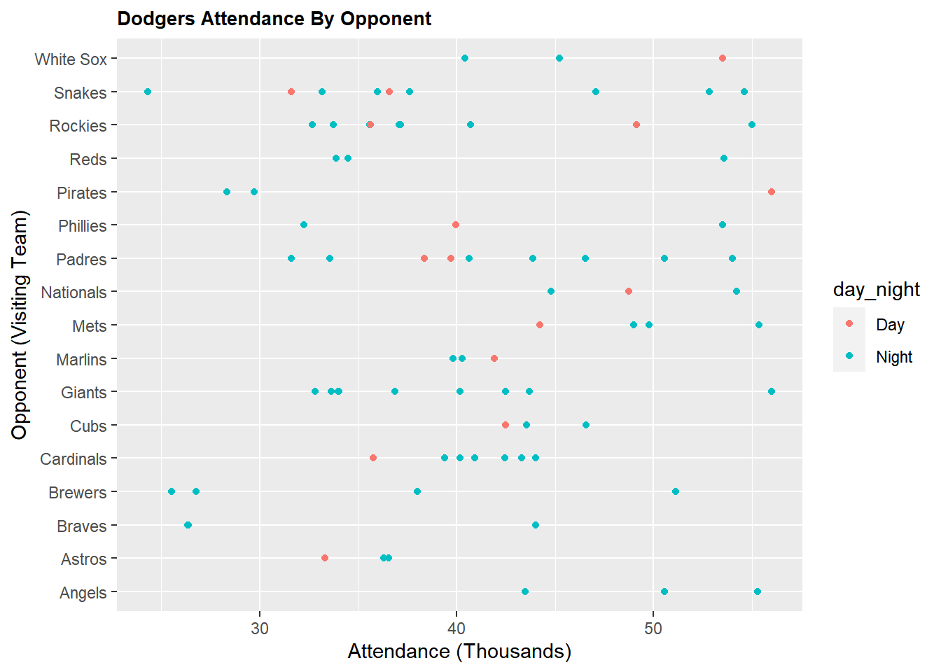

##Design Predictive Model

To advise the management if promotions impact attendance we will need to identify if there is a positive effect, and if there is a positive effect how much of an effect it is.

To provide this advice, I built a Linear Model for predicting attendance using Month, Day Of Week and the indicator variable Bobblehead promotion. I split the data into Training and Test to create the model

# Create a model with the bobblehead variable entered last
my.model <- {attend ~ month + day_of_week + bobblehead}

# use the full data set to obtain an estimate of the increase in
# attendance due to bobbleheads, controlling for other factors
my.model.fit <- lm(my.model, data = DodgersData)  # use all available data
print(summary(my.model.fit))

## 
## Call:
## lm(formula = my.model, data = DodgersData)
## 
## Residuals:
##      Min       1Q   Median       3Q      Max 
## -10786.5  -3628.1   -516.1   2230.2  14351.0 
## 
## Coefficients:
##                      Estimate Std. Error t value Pr(>|t|)    
## (Intercept)          38792.98    2364.68  16.405  < 2e-16 ***
## monthAUG              2377.92    2402.91   0.990   0.3259    
## monthJUL              2849.83    2578.60   1.105   0.2730    
## monthJUN              7163.23    2732.72   2.621   0.0108 *  
## monthMAY             -2385.62    2291.22  -1.041   0.3015    
## monthOCT              -662.67    4046.45  -0.164   0.8704    
## monthSEP                29.03    2521.25   0.012   0.9908    
## day_of_weekMonday    -4883.82    2504.65  -1.950   0.0554 .  
## day_of_weekSaturday   1488.24    2442.68   0.609   0.5444    
## day_of_weekSunday     1840.18    2426.79   0.758   0.4509    
## day_of_weekThursday  -4108.45    3381.22  -1.215   0.2286    
## day_of_weekTuesday    3027.68    2686.43   1.127   0.2638    
## day_of_weekWednesday -2423.80    2485.46  -0.975   0.3330    
## bobbleheadYES        10714.90    2419.52   4.429 3.59e-05 ***
## ---
## Signif. codes:  0 '***' 0.001 '**' 0.01 '*' 0.05 '.' 0.1 ' ' 1
## 
## Residual standard error: 6120 on 67 degrees of freedom
## Multiple R-squared:  0.5444, Adjusted R-squared:  0.456 
## F-statistic: 6.158 on 13 and 67 DF,  p-value: 2.083e-07

4.10 Reference

This case study is originally from Modeling Techniques in Predictive Analysis by Thomas W. Miller. Thank you, Dr. Miller!

This book a must-read for digital marketers!!! Enjoy and have fun!