Chapter 9 Hierarchical Cluster Analysis
9.1 Learning objectives
By the end of this lab session, you should be able to:
1. Understand how cloud computing works (currently in beta release at the time I am writing this tutorial).
2. Understand how hierarchical cluster analysis works.
3. Create descriptive stats to help understand the frequency distributions of your data
4. Perform a very basic cluster analysis and output the results of a basic geodemographic classification
5. Understand how to interpret your cluster analysis results.
6.Understand how to import your own data to the cloud environment
7.Understand how to export your final results from the cloud environment to your own computer
8.Understand how to use some basic packages and custom functions to process your data (optional)
Reading
For hierachical clustering and exploratory data analysis read Chapter 12 “Cluster Analysis” from An Introduction to Statistical Learning with Applications in R by Gareth James, Daniela Witten, Trevor Hastie and Robert Tibshirani - reading (p.385-p.399).
Remember this is just a starting point, explore the reading list, practical and lecture for more ideas.
Reference: Gareth James, Daniela Witten, Trevor Hastie and Robert Tibshirani 2013.An Introduction to Statistical Learning with Applications in R. https://faculty.marshall.usc.edu/gareth-james/ISL/ISLR%20Seventh%20Printing.pdf
Notice: This is still an early draft. Let me know if there are any errors or typos.
Keep in mind that no programmer can avoid errors. I strongly agree with this quote from “CodeAcademy” that “Errors in your code mean you’re trying to do something cool.”
9.2 Segmentation
Objective - Dividing the target market or customers on the basis of some significant features which could help a company sell more products in less marketing expenses.
A potentially interesting question might be are some products (or customers) more alike than the others.
9.3 Market segmentation
Market segmentation is a strategy that divides a broad target market of customers into smaller, more similar groups, and then designs a marketing strategy specifically for each group. Clustering is a common technique for market segmentation since it automatically finds similar groups given a data set.
9.4 Create a product which evokes the needs & wants in target market
Imagine that you are the Director of Customer Relationships at Apple, and you might be interested in understanding consumers’ attitude towards iPhone 12 and Google’s Pixel 5. Once the product is created, the ball shifts to the marketing team’s court. As mentioned above, to understand which groups of customers will be interested in which kind of features, marketers will make use of market segmentation strategy. The cluster analysis algorithm is designed to address this problem. Doing this ensures the product is positioned to the right segment of customers with a high propensity to buy.
9.5 Examples of Objectives
1.Identify the type of customers who would respond to a particular offer
2.Identify high spenders among customers who will use the e-commerce channel for festive shopping
3.Identify customers who will default on their credit obligation for a loan or credit card
9.6 Hierarchical clustering (single link) visuals/activity with creatures
9.7 Dataset
The file customer_segmetation.csv contains data collected by one of the student groups who took the marketing research course in spring 2020.
9.8 Importing data - No need to download R or R studio
Search for Rstudio Cloud, register (or set up a free user account), and log into the cloud environment with your Gmail credentials.
You will upload your dataset (.csv) from your own computer to R Studio Cloud first. Make sure the first column is id instead of a variable.
Once the dataset is uploaded, you will see the dataset available on the right pane of your cloud environment.
Now we will be using the package (readr) and the function read_csv to read the dataset.
library(readr)
mydata <-read_csv('https://raw.githubusercontent.com/utjimmyx/regression/master/customer_segmentation.csv')
## Rows: 22 Columns: 15
## -- Column specification --------------------------------------------------------
## Delimiter: ","
## dbl (15): ID, CS_helpful, Recommend, Come_again, Product_needed, Profesional...
##
## i Use `spec()` to retrieve the full column specification for this data.
## i Specify the column types or set `show_col_types = FALSE` to quiet this message.9.9 Importing data
In the following step, you will standardize your data(i.e., data with a mean of 0 and a standard deviation of 1). You can use the scale function from the R environment which is a generic function whose default method centers and/or scales the columns of a numeric matrix.
9.10 Building distance function and ploting the trees (dendrograms)
Hierarchical clustering (using the function hclust) is an informative way to visualize the data.
We will see if we could discover subgroups among the variables or among the observations.
use = scale(mydata[,-c(1)], center = TRUE, scale = TRUE)
dist = dist(use)
d <- dist(as.matrix(dist))   # find distance matrix
seg.hclust <- hclust(d)                # apply hirarchical clustering
library(ggplot2) # needs no introduction
plot(seg.hclust)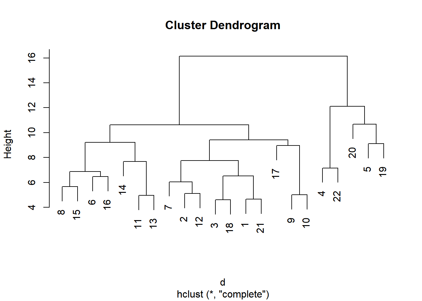
9.11 Identifying clustering memberships for each cluster
Imagine if your goal is to find some profitable customers to target. Now you will be able to see the number of customers using this algorithm.
groups.3 = cutree(seg.hclust,3)
table(groups.3)  #A good first step is to use the table function to see how # many observations are in each cluster
## groups.3
## 1 2 3
## 17 2 3#In the following step, we will find the members in each cluster or group.
mydata$ID[groups.3 == 1]## [1] 1 2 3 6 7 8 9 10 11 12 13 14 15 16 17 18 21mydata$ID[groups.3 == 2]## [1] 4 22mydata$ID[groups.3 == 3]## [1] 5 19 20Finding means or medians of each variable (factor) for each cluster
Imagine if your goal is to find some profitable customers to target. Now using the mean function or the median function, you will be able to see the characteristics of each sub-group. Now it is time to use your domain expertise.
9.11.1 We can look at the medians (or means) for the variables in each cluster - Questions for you - why?
9.11.2 How to get it done? You can get it done using Excel. However, it is too tedious
9.12 Advanced questions (optional)
The aggregate function is well suited for this task To see how the aggregate function works, please add ? to aggregate and see what happens Do you think if mean or median should be used? Why or why not?
Be very careful!!! Should we use mydata or mydata[,-1] along with the aggregate function? Why? Hint: see the results below:
#?aggregate
aggregate(mydata,list(groups.3),median)| Group.1 | ID | CS_helpful | Recommend | Come_again | Product_needed | Profesionalism | Limitation | Online_grocery | delivery | Pick_up | Find_items | other_shops | Gender | Age | Education |
|---|---|---|---|---|---|---|---|---|---|---|---|---|---|---|---|
| 1 | 11 | 1 | 1 | 1 | 2 | 1 | 1 | 2 | 2 | 3 | 1 | 2 | 1 | 2 | 2 |
| 2 | 13 | 3 | 2.5 | 1.5 | 3 | 1.5 | 2 | 3 | 3 | 2.5 | 2 | 1.5 | 1 | 2.5 | 5 |
| 3 | 19 | 2 | 1 | 3 | 3 | 2 | 1 | 2 | 3 | 1 | 2 | 3 | 2 | 2 | 2 |
aggregate(mydata,list(groups.3),mean)| Group.1 | ID | CS_helpful | Recommend | Come_again | Product_needed | Profesionalism | Limitation | Online_grocery | delivery | Pick_up | Find_items | other_shops | Gender | Age | Education |
|---|---|---|---|---|---|---|---|---|---|---|---|---|---|---|---|
| 1 | 10.8 | 1.29 | 1.12 | 1.24 | 1.82 | 1.24 | 1.35 | 2.24 | 2.24 | 2.71 | 1.29 | 2.65 | 1.18 | 2.41 | 3.12 |
| 2 | 13 | 3 | 2.5 | 1.5 | 3 | 1.5 | 2 | 3 | 3 | 2.5 | 2 | 1.5 | 1 | 2.5 | 5 |
| 3 | 14.7 | 2.33 | 1.67 | 2.67 | 3 | 2.33 | 2 | 2 | 3 | 1 | 2 | 3 | 2 | 2.67 | 2.33 |
aggregate(mydata[,-1],list(groups.3),median)| Group.1 | CS_helpful | Recommend | Come_again | Product_needed | Profesionalism | Limitation | Online_grocery | delivery | Pick_up | Find_items | other_shops | Gender | Age | Education |
|---|---|---|---|---|---|---|---|---|---|---|---|---|---|---|
| 1 | 1 | 1 | 1 | 2 | 1 | 1 | 2 | 2 | 3 | 1 | 2 | 1 | 2 | 2 |
| 2 | 3 | 2.5 | 1.5 | 3 | 1.5 | 2 | 3 | 3 | 2.5 | 2 | 1.5 | 1 | 2.5 | 5 |
| 3 | 2 | 1 | 3 | 3 | 2 | 1 | 2 | 3 | 1 | 2 | 3 | 2 | 2 | 2 |
aggregate(mydata[,-1],list(groups.3),mean)| Group.1 | CS_helpful | Recommend | Come_again | Product_needed | Profesionalism | Limitation | Online_grocery | delivery | Pick_up | Find_items | other_shops | Gender | Age | Education |
|---|---|---|---|---|---|---|---|---|---|---|---|---|---|---|
| 1 | 1.29 | 1.12 | 1.24 | 1.82 | 1.24 | 1.35 | 2.24 | 2.24 | 2.71 | 1.29 | 2.65 | 1.18 | 2.41 | 3.12 |
| 2 | 3 | 2.5 | 1.5 | 3 | 1.5 | 2 | 3 | 3 | 2.5 | 2 | 1.5 | 1 | 2.5 | 5 |
| 3 | 2.33 | 1.67 | 2.67 | 3 | 2.33 | 2 | 2 | 3 | 1 | 2 | 3 | 2 | 2.67 | 2.33 |
cluster_means <- aggregate(mydata[,-1],list(groups.3),mean)Export cluster analysis results into excel from R Studio Cloud
write.csv(groups.3, "clusterID.csv")
write.csv(cluster_means, "cluster_means.csv")
9.13 Downloading your results mannually
First, select the files (“clusterID.csv” & “cluster_means.csv”) and put a checkmark before each file.
Second, click the gear icon on the right side of your pane and export the data.
9.14 References
Cluster analysis - reading (p.385-p.399) https://faculty.marshall.usc.edu/gareth-james/ISL/ISLR%20Seventh%20Printing.pdf
Comparison of similarity coefficients used for cluster analysis with dominant markers in maize (Zea mays L) https://www.scielo.br/scielo.php?script=sci_arttext&pid=S1415-47572004000100014&lng=en&nrm=iso
Principal Component Methods in R: Practical Guide http://www.sthda.com/english/articles/31-principal-component-methods-in-r-practical-guide/118-principal-component-analysis-in-r-prcomp-vs-princomp/