第 2 章 R in OLS
2.1 參考資料
R magrittr 套件:在 R 中使用管線(Pipe)處理資料流 - G. T. Wang. (2016). G. T. Wang. Retrieved 5 March 2019, from https://blog.gtwang.org/r/r-pipes-magrittr-package/
2.2 setup
library("AER")
library("ggplot2")
library("dplyr")
library("knitr")
2.3 dataframe物件
data("Journals")Journal這個dataframe的結構(structure)是什麼?有幾個變數?每個變數物件的類別(class)又是什麼?
找出Journal資料的詳細說明。
2.4 資料處理:產生新變數 dplyr::mutate
Journals %>% mutate(citeprice=price/citations) -> journals
summary(journals)
2.5 因果問句
期刊的價格(citeprice,平均文獻引用價格)如何影響其圖書館訂閱量(subs)?
library(psych)
journals %>%
  select(citeprice,subs) %>%
  pairs.panels()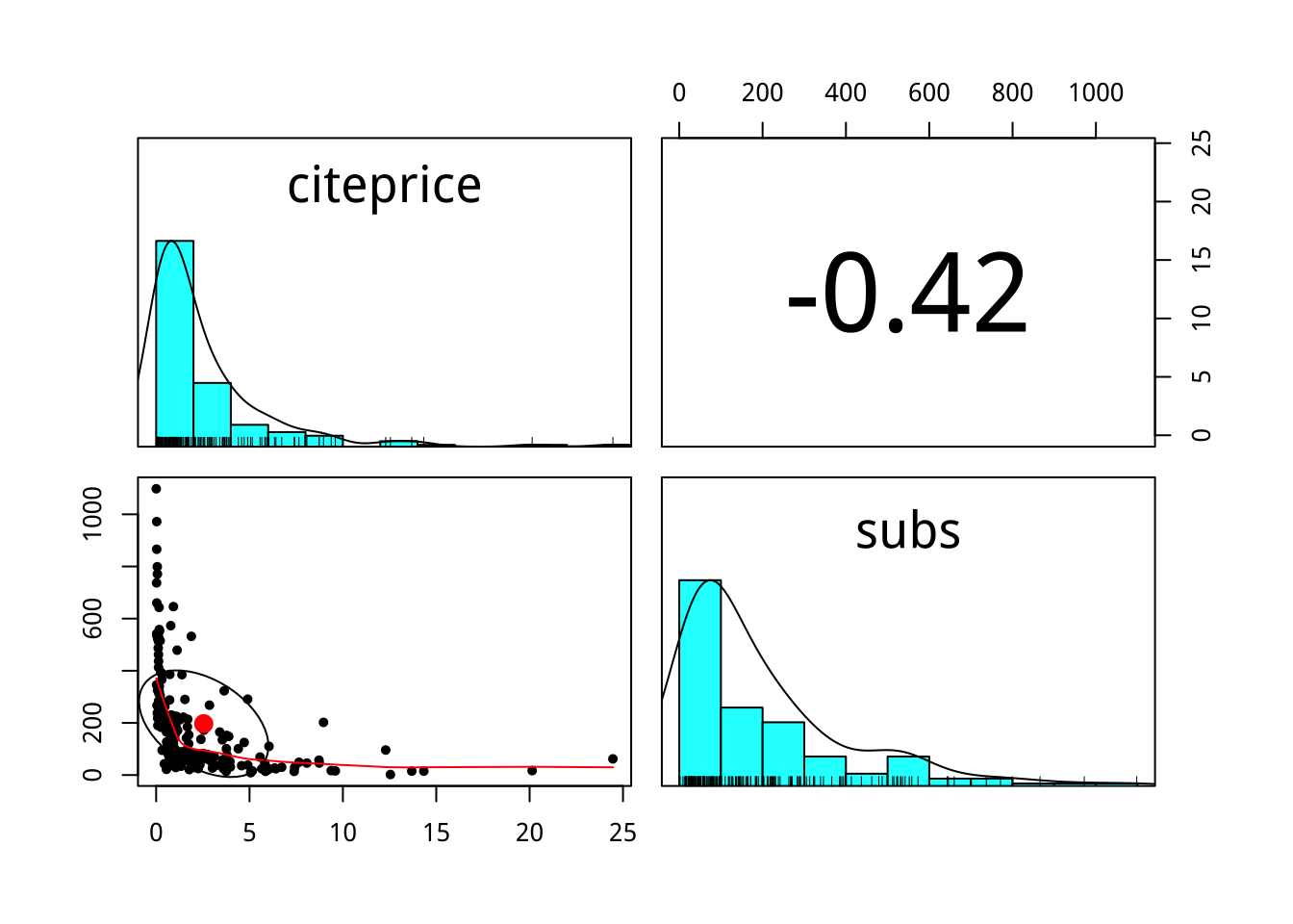
journals %>%
  select(citeprice,subs) %>%
  mutate_all(log) %>%
  pairs.panels()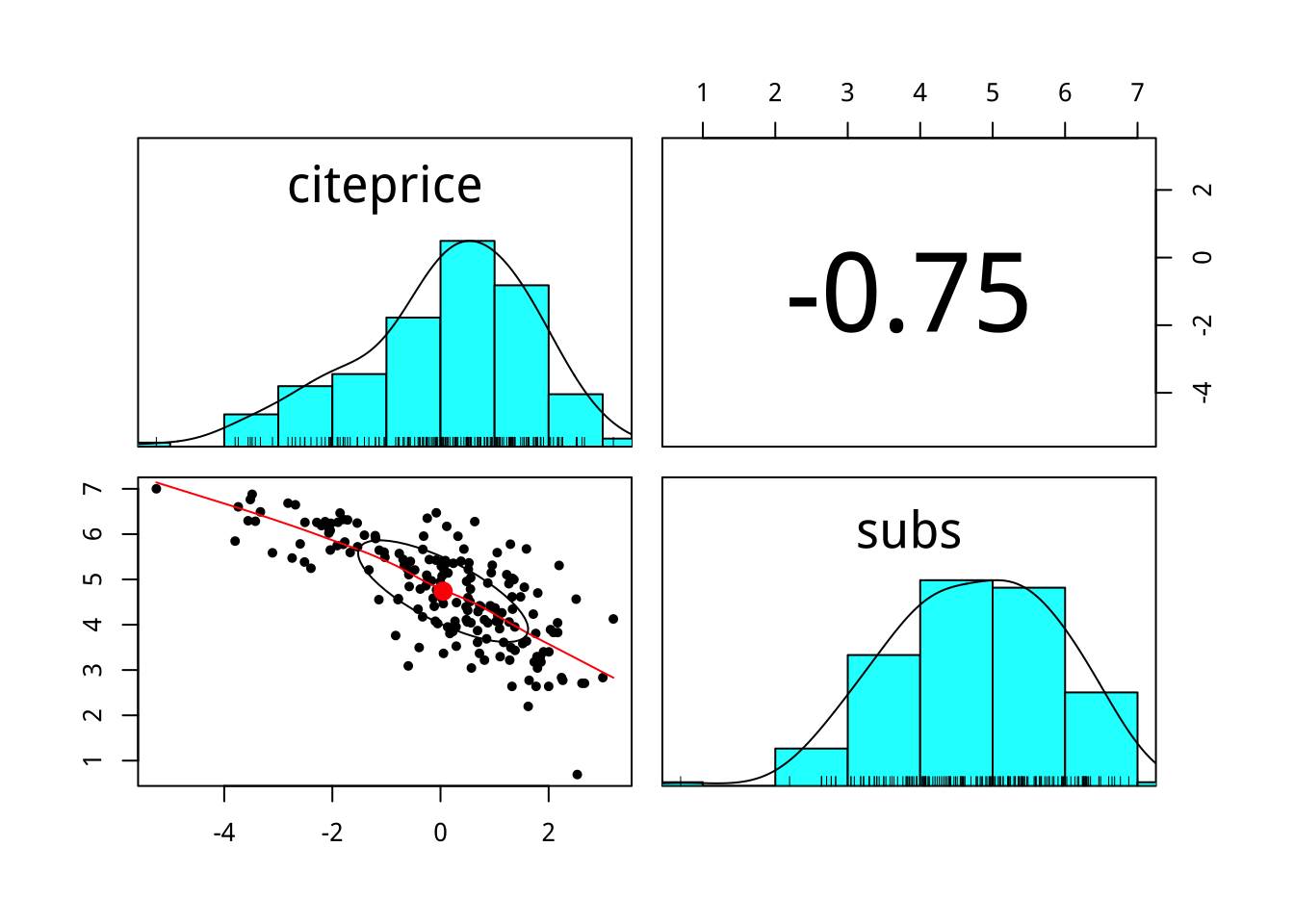
為什麼取log後,兩者的相關度變高?它表示兩個變數變得更不獨立嗎?
2.6 效應評估
當解釋變數並非直接代表有沒有受試的dummy variable(即只有0或1可能值)時,可以用以下的間斷例子來思考迴歸模型的係數含意:
假設\(P_i\)就只有高價(\(P_H\))及低價(\(P_L\))兩種,\(Y_{Hi},Y_{Li}\)分別代表期刊\(i\)在在高價及低價的訂閱量,我們觀察到的訂量\(Y_i\)只會是\(Y_{Hi},Y_{Li}\)其中一個。我們可以將\(Y_i\)與\(P_i\)寫成如下的效應關係:
\[Y_i=Y_{Li}+\frac{Y_{Hi}-Y_{Li}}{P_H-P_L}(P_i-P_L)\]
若假設價格對每個期刊帶來的單位變化固定,即: \[\frac{Y_{Hi}-Y_{Li}}{P_H-P_L}=\beta_1^*\]
則 \[Y_i=Y_{Li}+\beta_1^*(P_i-P_L)\]
單純比較不同「期刊價格」(citeprice)的期刊所獨得的圖書館「訂閱數」(subs)變化並無法反應真正的「期刊價格」效應,原因是「立足點」並不與「期刊價格」獨立。
這裡「立足點」指得是什麼?
「低價格下的訂閱數」(包含高價格期刊若採低價格的訂閱情境)。
你認為高價期刊,若採低價,它的訂閱數會與目前低價期刊相同嗎?為什麼?
2.7 進階關連分析
數值變數v.s.數值變數
# 判斷變數是否為數值類別
is_numeric<-function(x) all(is.numeric(x))
# 計算數數與citeprice的相關係數
cor_citeprice<-function(x) cor(x,journals$citeprice)

journals %>%
  select_if(is_numeric) %>%
  summarise_all(cor_citeprice) %>%
  kable()
期刊越重要,其引用次數越高,因此高引用次數的期刊,你認為它在「低價格下的訂閱數」(立足點)會比較高還是低?
承上題,單純比較「期刊引用單價」高低間的「訂閱數量」差別,所估算出來的價格效果以絕對值來看會高估、還是低估?為什麼?
2.8 複迴歸模型
journals %>%
  lm(log(subs)~log(citeprice),data=.) -> model1

journals %>%
  lm(log(subs)~log(citeprice)+foundingyear,data=.) -> model2
2.9 broom
tidy()
augment()
glance()
library(broom)tidy(model1)## # A tibble: 2 x 5
## term estimate std.error statistic p.value
## <chr> <dbl> <dbl> <dbl> <dbl>
## 1 (Intercept) 4.77 0.0559 85.2 2.95e-146
## 2 log(citeprice) -0.533 0.0356 -15.0 2.56e- 33augment(model1)## # A tibble: 180 x 9
## log.subs. log.citeprice. .fitted .se.fit .resid
## <dbl> <dbl> <dbl> <dbl> <dbl>
## 1 2.64 1.77 3.82 0.0829 -1.18
## 2 4.08 -0.0953 4.82 0.0561 -0.739
## 3 2.83 3.00 3.17 0.119 -0.332
## 4 0.693 2.53 3.42 0.105 -2.72
## 5 4.56 2.51 3.43 0.104 1.14
## 6 2.71 2.66 3.35 0.109 -0.639
## 7 2.64 1.32 4.06 0.0720 -1.42
## 8 5.31 2.19 3.60 0.0946 1.71
## 9 3.83 2.09 3.65 0.0917 0.176
## 10 3.83 2.17 3.61 0.0939 0.218
## # … with 170 more rows, and 4 more variables:
## # .hat <dbl>, .sigma <dbl>, .cooksd <dbl>,
## # .std.resid <dbl>glance(model1)## # A tibble: 1 x 11
## r.squared adj.r.squared sigma statistic p.value
## <dbl> <dbl> <dbl> <dbl> <dbl>
## 1 0.557 0.555 0.750 224. 2.56e-33
## # … with 6 more variables: df <int>, logLik <dbl>,
## # AIC <dbl>, BIC <dbl>, deviance <dbl>,
## # df.residual <int>2.10 模型比較
journals %>%
  lm(log(subs)~log(citeprice),data=.) -> model_1
journals %>%
  lm(log(subs)~log(citeprice)+foundingyear,data=.) -> model_2

library(sandwich)
library(lmtest)
library(stargazer)

#使用vcovHC函數來計算HC1型的異質變異(即橫斷面資料下的線性迴歸模型)
coeftest(model_1, vcov. = vcovHC, type="HC1") -> model_1_coeftest
coeftest(model_2, vcov. = vcovHC, type="HC1") -> model_2_coeftest

stargazer(model_1, model_2,
          se=list(model_1_coeftest[,"Std. Error"], model_2_coeftest[,2]),
          type="html",
align=TRUE)關於vcovHC()更多type的探討,請見:
Zeileis A (2006), Object-Oriented Computation of Sandwich Estimators. Journal of Statistical Software, 16(9), 1–16. URL http://www.jstatsoft.org/v16/i09/.