10 Retirement Strategies
Continuing in the vein of building upon and improving previously written functions, a “Retirement Strategies” page was envisioned. Four theoretical strategies were modelled:
- 100% Annuity: An annuity is purchased with the retirement fund
- 100% Drawdown: The retirement fund is drawn down for remainder of retiree’s life
- Drawdown and Annuity Purchase: The initial fund is drawn down for a specified period. The resulting fund value is used to purchase an annuity
- Drawdown and Deferred Annuity: A deferred annuity is purchased at retirement. It gives the same payment as the 100% Annuity strategy. The remainder of the retirement fund is drawn down for the deferment period
It is difficult to compare these four strategies, as it is not a like-for-like comparison. These strategies were envisioned primarily as a demonstration of the building-block nature of the R code underpinning this Shiny application - the first two strategies are very similar to those seen in the combined SORP and Drawdown Calculator, and the last two strategies were both modelled using a combination of the functions built for the SORP Calculator and the Drawdown Simulator.
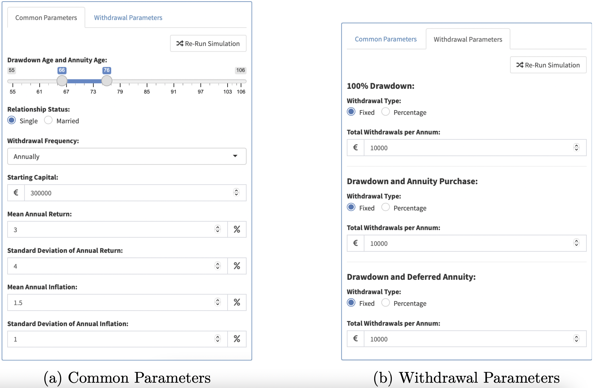
Figure 10.1: Inputs
Two tabs of Parameters are displayed (Figure 10.1). The Common Parameters (Figure 10.1a) resemble the Drawdown Simulator’s inputs, with a few key differences. First, an “Annuity Age” must be specified - this is the age at which the third and fourth strategies switch from Drawdown to an Annuity. A relationship status is also required, to aid in the pricing of annuities. Finally, the “Withdrawal Type/Amount” inputs are moved to a separate tab (Figure 10.1b), so as to enable the user to trial differing withdrawal strategies for different retirement products. Once again, a Re-Run Simulation Button is provided on each tab.
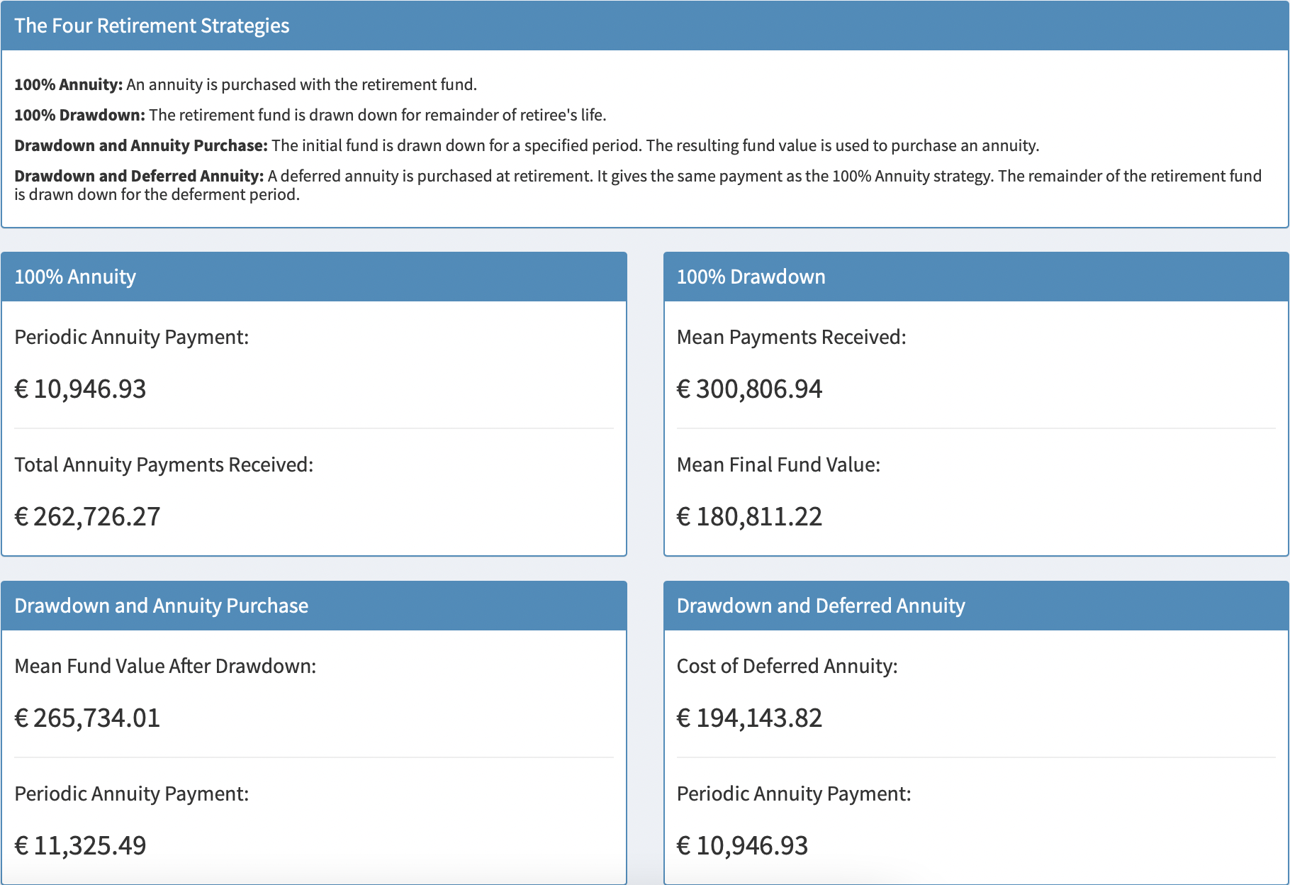
Figure 10.2: Information Box & Key Figures
As there are now four different strategies being showcased on this page, an information box is vital to make sure that the user understands what is actually on display. Underneath this box, a number of key figures for each strategy are shown (Figure 10.2).
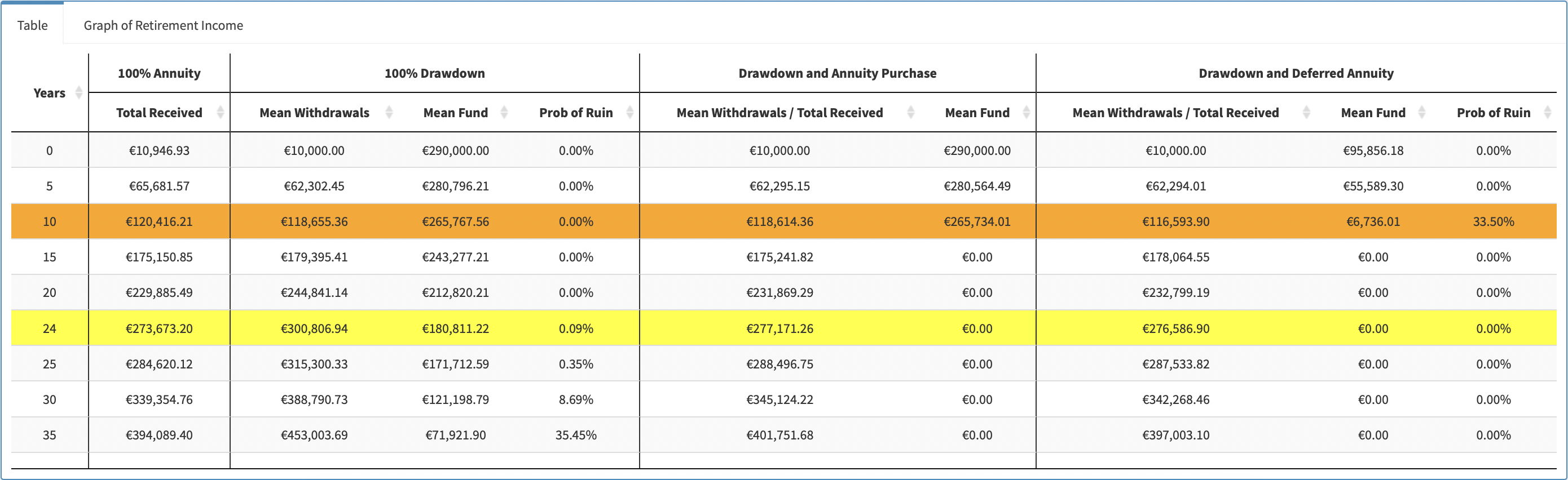
Figure 10.3: Table
Sitting underneath both the parameters panel and the summary output is a tabBox with two panels: Firstly, a summary table (Figure 10.3) is generated using DT [8]. This table once again builds upon its predecessors. An orange row is inserted to signal the switch from drawdown to annuity strategies, and a yellow row is inserted at the life expectancy. This table is a more fleshed-out display of the key figures outlined above.
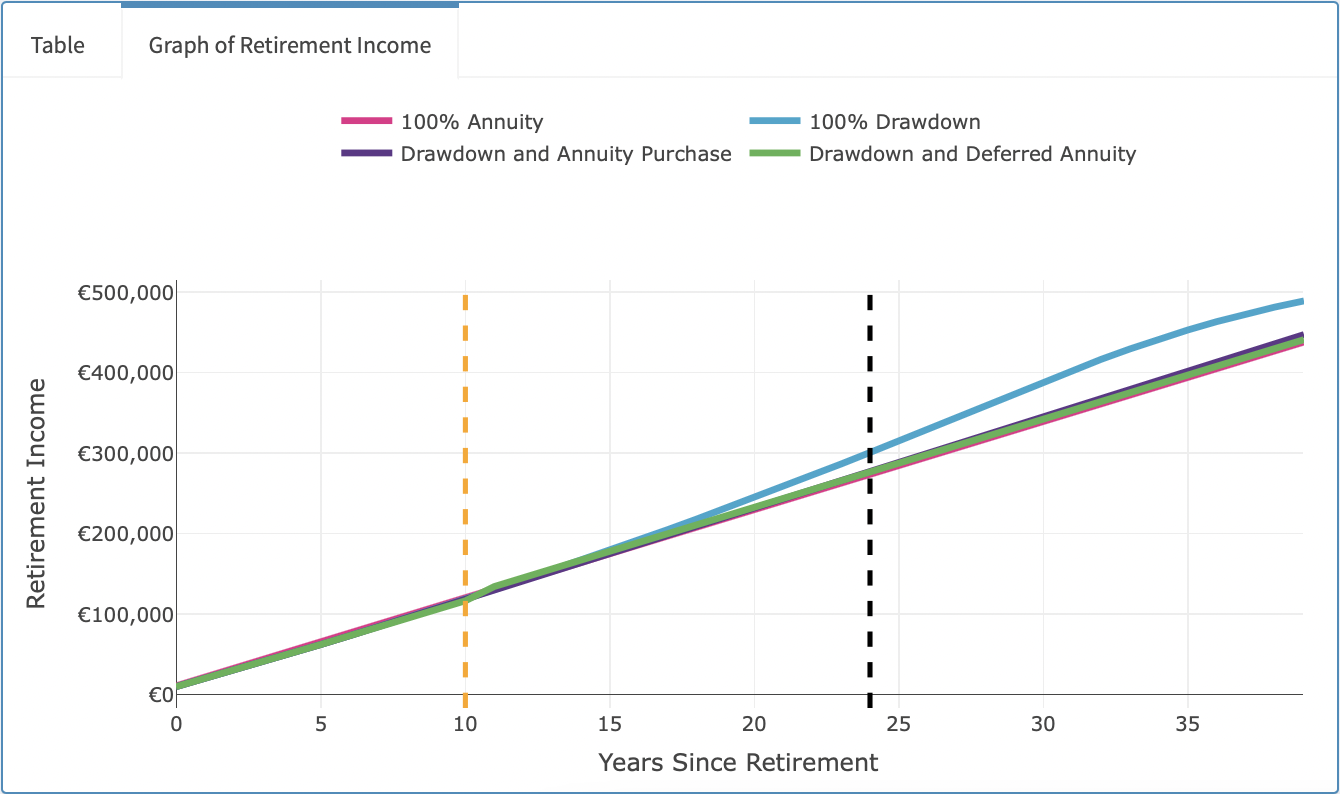
Figure 10.4: Graph of Retirement Income
Finally, a graph showing the mean retirement income received over time is created in the other panel of the tabBox (Figure 10.4). The ‘switch-over age’ is indicated by the orange dashed line, and the life expectancy is once again shown in black. This graph is also created in Plotly [12], so as to allow the user to see the mean retirement income they can expect to receive from each strategy at any given time point (Figure 10.5).
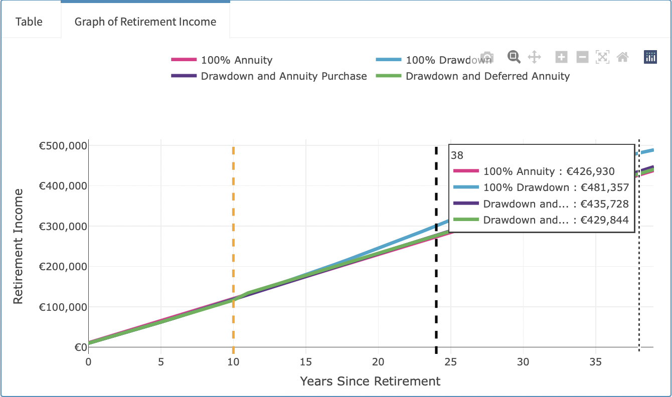
Figure 10.5: Graph of Retirement Income, with Plotly Hover Demonstration
The Retirement Strategies page is truly the culmination of this building-block approach to coding that R facilitates - by starting with two ‘simpler’ functionalities, it became possible to build other pages that became greater than the sum of their parts.