8 Drawdown Simulator
An increasingly prominent decision people face is whether to buy an annuity or draw down their pension at retirement. Drawdown, known as an Approved Retirement Fund (ARF) in Ireland [34], consists of keeping one’s pension savings invested with their pension provider when they reach retirement. Then each year, they decide how much money to take out of their pension pot to live on. The pension fund stays invested, usually in the stock market.
As a result, investment growth can provide higher returns and see the savings continue to increase in value. On the other hand, there is a risk that the fund may fall in value if the markets perform poorly. As such, income is not guaranteed for life. In essence, drawdown is a juggling act - one aims to balance taking out enough cash for a comfortable retirement, while keeping enough invested to provide for later years.
Benefiting from the open-source nature of R, code sourced on the Systematic Investor Blog [35] was modified to build the Drawdown Simulator. 10,000 different simulations are run each time based on the parameters entered by the user, and these simulations are used to calculate reasonable estimates of future fund values, withdrawal amounts, and ruin probabilities.
In a similar style to the SORP Calculator (Figure 6.1), the Drawdown Simulator uses a Sidebar Layout. The user enters their age, the value of their fund upon retirement, and see how the size, type and frequencies of withdrawals affect their wealth (Figure 8.1). There are two withdrawal types, both adjusted for inflation - a fixed withdrawal amount per annum, or a percentage of the starting fund value (this option is provided to help the user easily model withdrawal strategies similar to the “4% Rule” [36]). The user is able to select which type of withdrawal they wish to simulate, and only the appropriate input box is then displayed (utilising shinyjs [6]) so as to avoid confusion.
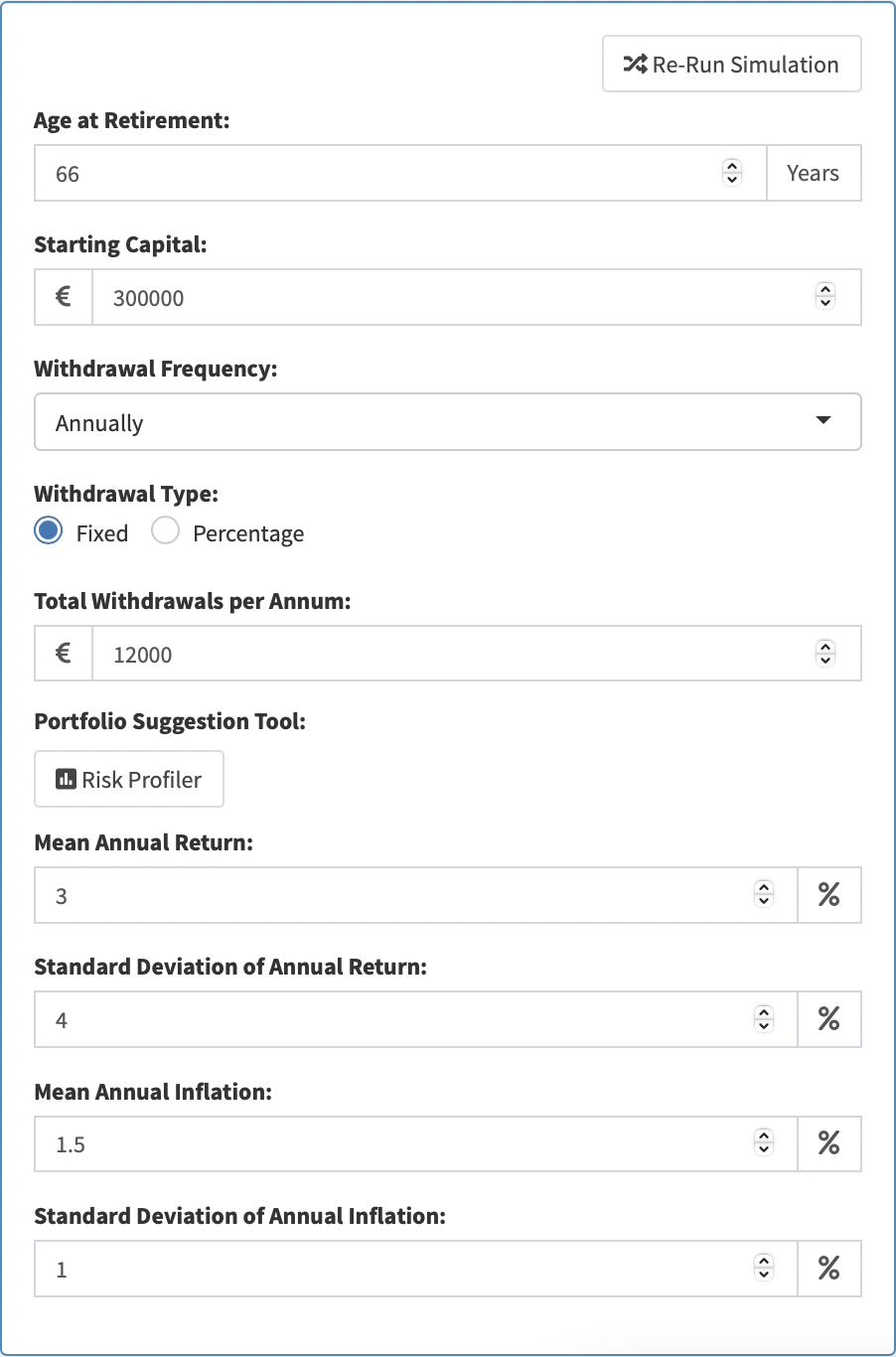
Figure 8.1: Parameters
The change in the pension fund over time is simulated using periodic investment returns, inflation and withdrawals. The investment and inflation returns are randomly generated from the normal distribution incorporating their associated means and standard deviations, as inputted by the user.3
Due to the time necessary to run all these computations, instead of updating dynamically like the Loan and SORP Calculators, for the Drawdown Simulator a “Re-Run Simulation” button was added, so that when the user is satisfied with their parameters, then can make all their changes at once, rather than unnecessarily running many simulations at a time.
Based on the parameters entered, the app first displays three key metrics for the user in information boxes: their life expectancy (based on the ILT15 Life Tables [37], which were utilised as part of the SORP assumptions), the median fund value at their life expectancy, and the probability of ruin at their life expectancy (Figure 8.2).
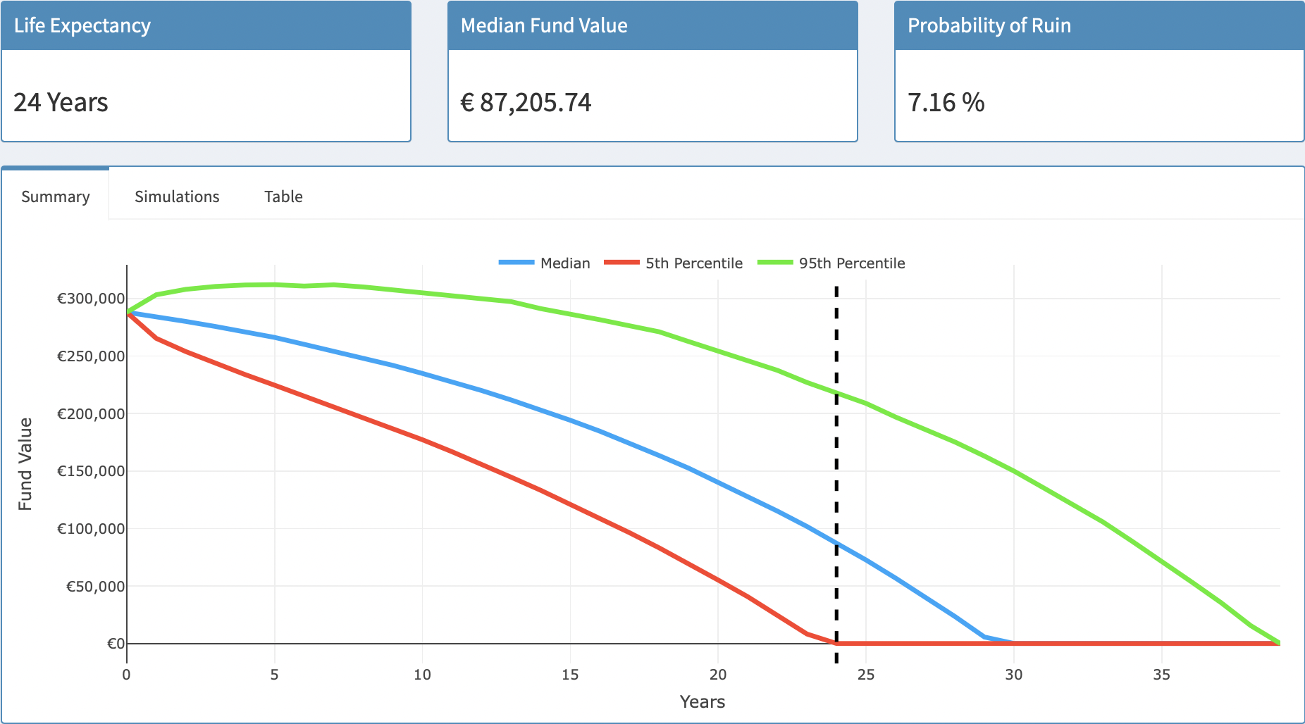
Figure 8.2: Key Metrics & Summary Graph
Underneath these key outputs, a tab-box is generated, with three different displays of summary data. Firstly, an interactive summary graph is created. It displays the 5th percentile, 95th percentile, and median fund values for each time-point (Figure 8.3). This graph was coded using Plotly, an R Library that allows for the user to interact with graphs. In this instance, the user can hover over the graph to see exact figures for each time point. A custom function was also created so that the user’s life expectancy is shown on the graph as a dashed black line. This allows the user to visualise how their withdrawal decisions affect them in both a optimistic and pessimistic scenario, both from an investment and a mortality risk point of view.
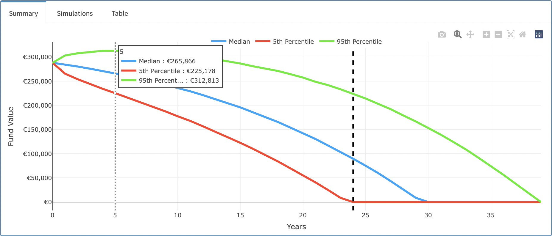
Figure 8.3: Summary Graph, with Plotly Hover Demonstration
Next, the first 25 of the 10,000 drawdown simulations are plotted, with the life expectancy once again indicated (Figure 8.4). This is to give the user an indication of possible paths of how their fund could progress over time, while also serving as an illustration of the powerful stochastic simulations being carried out in the background.
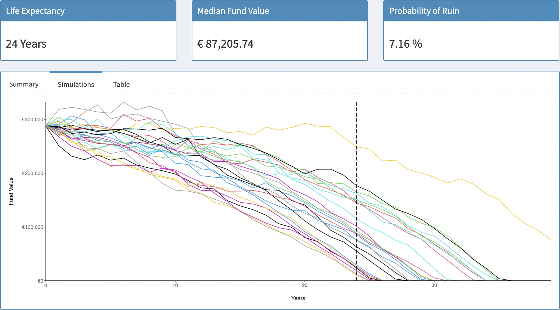
Figure 8.4: Simulations
Finally, a table is generated (Figure 8.5), showing key data at five-yearly intervals, with the data at the life expectancy highlighted. The mean cumulative withdrawals and fund value are displayed, along with the probability of ruin by that time point, and the 5th/50th/95th Percentiles of Fund Values.
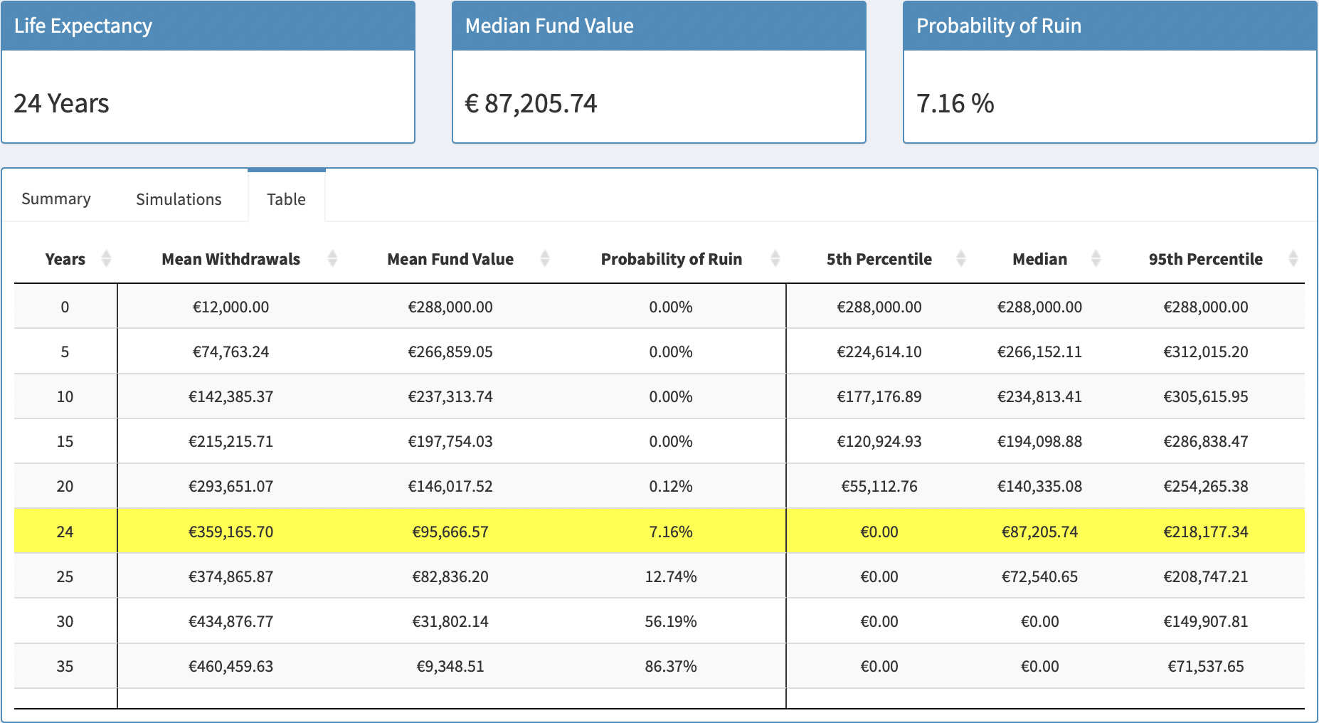
Figure 8.5: Table
This simulator is a fantastic demonstration of the highlights of what R has to offer: great flexibility in parameters, stochastic modelling, powerful simulations, and exemplary graphical capabilities.
A “Risk Profiler” interactive tool to determine a user’s appetite for risk is also included on this page, however this tool is outside the scope of this report.↩︎