Chapter 2 R

“We can’t overestimate the value of computers.” -Michael Scott

Motivation

For many Statistical topics - and especially in Stochastic Processes - using computers can help us to explore different topics to their fullest extent. In this book, we will be working with the statistical programming language R (indeed, these words are written in ‘R Markdown,’ with the help of this excellent resource). We will be reviewing some of the more advanced techniques that R leverages; please see this review for other starting material.

2.1 Applies

Apply functions like sapply, apply and lapply allow us to, well apply a function over an object (i.e., a vector, list, etc.) in R. Using an apply can often be cleaner, easier, and (sometimes) marginally faster than for loops (we won’t be working with truly large datasets so we won’t be overly focused on processing speed). The setup is relatively simple, and we will start with sapply, which just stands for ‘simplify apply.’

# define a vector
x <- 1:10

# apply the square function over the vector
sapply(x, function(x) x ^ 2)

##  [1]   1   4   9  16  25  36  49  64  81 100

The first argument is simply the object, and the second argument is the function we want to apply over the object. Here we use the square function, so we write function(x) x ^ 2, which tells sapply to apply a function that takes input x and returns output x ^ 2.

It is important to note that, for an operation like this, taking advantage of R’s vectorization (ability to automatically apply a function over a vector or other object) would be quicker. We can see that here, by using Sys.time() to measure how long our code takes to run.

# sapply solution
start <- Sys.time()
sapply(x, function(x) x ^ 2)

##  [1]   1   4   9  16  25  36  49  64  81 100

print(Sys.time() - start)

## Time difference of 0.007485151 secs

# vectorization solution
start <- Sys.time()
x ^ 2

##  [1]   1   4   9  16  25  36  49  64  81 100

print(Sys.time() - start)

## Time difference of 0.00357914 secs

However, there are times when sapply can be useful. Imagine if you had a vector of 1000 random letters (you can always access this in R via the object letters) and wanted to create a numeric vector that had value 1 if the corresponding letter in your letter vector was a vowel and 0 if it was a consonant. Here, we can make use of sapply (we use the head function to check the first few entries in the output):

# sample letters:
samp_letters <- sample(letters, size = 1000, replace = TRUE)

# sapply solution
start <- Sys.time()
head(sapply(samp_letters, function(x) {
            if (x %in% c("a", "e", "i", "o", "u")) return(1)
            return(0)
            }))

## r e n a m y 
## 0 1 0 1 0 0

print(Sys.time() - start)

## Time difference of 0.0180819 secs

We can use apply and lapply for similar applications, just with different objects. For example, apply works on arrays or matrices. We merely need to specify if we need to apply the function over the rows (we enter 1 as the second argument) or the columns (we enter 2 as the second argument).

We can test apply by setting up a matrix of random data and then, for example, finding the value in the 95th percentile of each row.

# generate data
x <- matrix(rnorm(1000 * 100),
            nrow = 1000,
            ncol = 100)

# apply 95th percentile function
head(apply(x, 1, function(x) quantile(x, .95)))

## [1] 1.444122 1.389540 1.635034 1.575703 1.824760 1.427398

If we wanted to apply that same function over the columns of the matrix, we would simply use 2 in the second argument instead of 1.

Finally, lapply works in the same way but on lists. A quick refresher on lists; they are R objects that contain different elements which may be different ‘types’ (numerics, strings, etc.). Essentially, they allow us to group together things that might not be the same type. If we use the more common concatenate c, we get some strange results when we mix types:

c(4, "hello")

## [1] "4"     "hello"

Notice that concatenating a numeric, 4, which a string, hello, converts 4 to a string so that the two types match. Obviously, this would not be helpful if we wanted to maintain that 4 was a numeric; lists are helpful in this regard.

x <- list(4, "hello", rnorm(5))
x[[1]]

## [1] 4

x[[2]]

## [1] "hello"

x[[3]]

## [1] -0.3552938  0.7640098  0.3007766  0.8413623 -0.2883009

Note that the list maintains the type of the inputs; 4 and the rnorm(5) output are still numeric, while hello is still a string. Also note that we can index into a list with x[[i]] (this just grabs the $i^{th}$ element in the list).

Let’s try using lapply, then, to simply find the type of all of the elements in a list (which we can do with the function class).

x <- list(4, "hello", rnorm(5))
lapply(x, class)

## [[1]]
## [1] "numeric"
## 
## [[2]]
## [1] "character"
## 
## [[3]]
## [1] "numeric"

2.2 data.table

There are many handy objects for storing data in R; you’ve probably grown accustomed to using data.frame, matrix and similar functions. The data.table object (available, of course, in the data.table package) is especially popular and useful.

Since this isn’t a data science book, we won’t be covering the deep intricacies of the package; some of the complexities are explored in this vignette. Let’s start with actually defining a data.table:

library(data.table)
data <- data.table(letter = letters,
                   score = rnorm(26))
head(data)

##    letter      score
## 1:      a -0.5723140
## 2:      b -0.5395135
## 3:      c  0.8182038
## 4:      d -1.2698973
## 5:      e -1.0723506
## 6:      f  1.5048800

This might be a dataset on, say, how much someone likes each letter in the alphabet (they assign a numerical score based on how much they like the letter).

The $ operator allows us to access individual columns of the data.table:

head(data$letter)

## [1] "a" "b" "c" "d" "e" "f"

mean(data$score)

## [1] 0.1569299

We can also easily index into any row of the data.table:

# grab 17th row
data[17]

##    letter    score
## 1:      q 1.209325

# grab 'm' row
data[which(letter == "m")]

##    letter     score
## 1:      m -1.981792

We can even index into a specific row and column:

# grab 23rd row, 2nd column
data[23, 2]

##        score
## 1: -2.118373

It’s very easy to add a column with the $ and to remove it by setting the column to NULL:

# add column...
data$score_sq <- data$score ^ 2
head(data)

##    letter      score  score_sq
## 1:      a -0.5723140 0.3275433
## 2:      b -0.5395135 0.2910748
## 3:      c  0.8182038 0.6694575
## 4:      d -1.2698973 1.6126392
## 5:      e -1.0723506 1.1499358
## 6:      f  1.5048800 2.2646639

# ...and remove it
data$score_sq <- NULL
head(data)

##    letter      score
## 1:      a -0.5723140
## 2:      b -0.5395135
## 3:      c  0.8182038
## 4:      d -1.2698973
## 5:      e -1.0723506
## 6:      f  1.5048800

If you don’t like the $ operator, data.table even has a built in way to add columns with the := operator. Simply put the name of the new column (score_sq here) in front of the := operator and put the value of the new column after the operator (here, score ^ 2). By leaving the first argument (before the ,) empty in data[], we are telling data.table to perform this calculation for all rows. Similar to the $ operator, we can use NULL to remove columns.

data[ , score_sq := score ^ 2]
head(data)

##    letter      score  score_sq
## 1:      a -0.5723140 0.3275433
## 2:      b -0.5395135 0.2910748
## 3:      c  0.8182038 0.6694575
## 4:      d -1.2698973 1.6126392
## 5:      e -1.0723506 1.1499358
## 6:      f  1.5048800 2.2646639

data[ , score_sq := NULL]
head(data)

##    letter      score
## 1:      a -0.5723140
## 2:      b -0.5395135
## 3:      c  0.8182038
## 4:      d -1.2698973
## 5:      e -1.0723506
## 6:      f  1.5048800

It’s also easy to use the := operator to change existing values in the table instead of adding an entirely new column. We can use the first argument in data[] to select the correct row, then use an existing column (here, score) before the := operator to set a new value:

# change 'f' row to zero
data[letter == "f", score := 0]
data[letter == "f"]

##    letter score
## 1:      f     0

We can quickly order the data.table by employing the order function:

head(data[order(score, decreasing = TRUE)])

##    letter    score
## 1:      l 2.166953
## 2:      x 1.867895
## 3:      t 1.667792
## 4:      z 1.340374
## 5:      v 1.304526
## 6:      q 1.209325

There are many more nifty things that you can do with data.table, but they are perhaps better suited for a data science book (check out the vignette linked above for more). We’ve covered a strong base here, and will be sure to work through any examples with any odd applications. The final benefit is that data.table objects will be very useful for our purposes: they work well with the ggplot2 visual suite, for instance (more on that to come!).

2.3 time series

Working with time series data - simply data over time - is usually a fundamental part of any practical statistical endeavor. Working with dates can be frustrating but, luckily, R provides plenty of tools to ease the load.

The xts package is one of the more popular time series packages in R.

We can initialize a time series simply with data and a vector of dates (which we specify with the order.by argument:

# replicate
set.seed(0)

# generate data
y <- 1:10 + rnorm(10)

# date vector
x <- seq(from = Sys.Date() - 9, to = Sys.Date(), by = 1)

# create time series
data <- xts(y, order.by = x)
data

##                 [,1]
## 2021-07-14  2.262954
## 2021-07-15  1.673767
## 2021-07-16  4.329799
## 2021-07-17  5.272429
## 2021-07-18  5.414641
## 2021-07-19  4.460050
## 2021-07-20  6.071433
## 2021-07-21  7.705280
## 2021-07-22  8.994233
## 2021-07-23 12.404653

We can access the dates in a time series by employing the index function (which simply asks for the ‘index’ of a time series):

index(data)

##  [1] "2021-07-14" "2021-07-15" "2021-07-16" "2021-07-17" "2021-07-18" "2021-07-19"
##  [7] "2021-07-20" "2021-07-21" "2021-07-22" "2021-07-23"

Base R is also pretty good at plotting these xts objects:

plot(data)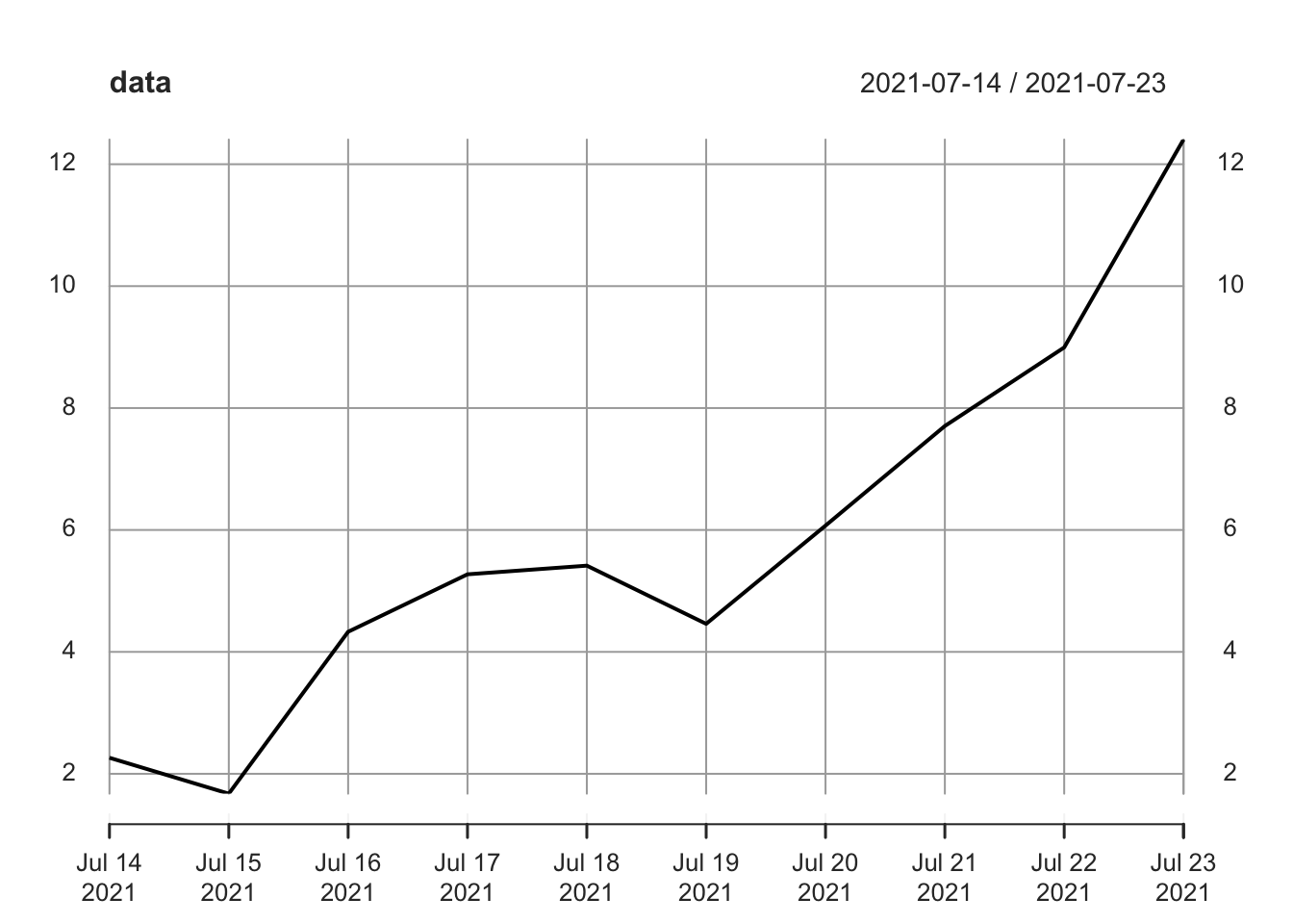

The above example was a univariate time series, but we can easily forge a multivariate time series by inputting multivariate data into xts:

# replicate
set.seed(0)

# generate data
y <- 1:10 + rnorm(10)
z <- 1:10 + rnorm(10)

# date vector
x <- seq(from = Sys.Date() - 9, to = Sys.Date(), by = 1)

# create time series
data <- cbind(y, z)
data <- xts(data, order.by = x)
data

##                    y        z
## 2021-07-14  2.262954 1.763593
## 2021-07-15  1.673767 1.200991
## 2021-07-16  4.329799 1.852343
## 2021-07-17  5.272429 3.710538
## 2021-07-18  5.414641 4.700785
## 2021-07-19  4.460050 5.588489
## 2021-07-20  6.071433 7.252223
## 2021-07-21  7.705280 7.108079
## 2021-07-22  8.994233 9.435683
## 2021-07-23 12.404653 8.762462

We can still easily generate a plot of this data:

plot(data)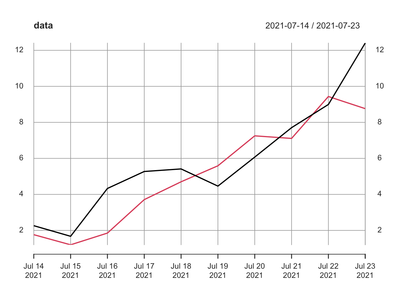

And access the dates with index:

index(data)

##  [1] "2021-07-14" "2021-07-15" "2021-07-16" "2021-07-17" "2021-07-18" "2021-07-19"
##  [7] "2021-07-20" "2021-07-21" "2021-07-22" "2021-07-23"

Finally, if we want to access the individual variables, we can do so with the $ operator. We can recover the actual numeric vector with the as.numeric function:

# grab y time series
data$y

##                    y
## 2021-07-14  2.262954
## 2021-07-15  1.673767
## 2021-07-16  4.329799
## 2021-07-17  5.272429
## 2021-07-18  5.414641
## 2021-07-19  4.460050
## 2021-07-20  6.071433
## 2021-07-21  7.705280
## 2021-07-22  8.994233
## 2021-07-23 12.404653

# grab numeric vector
as.numeric(data$y)

##  [1]  2.262954  1.673767  4.329799  5.272429  5.414641  4.460050  6.071433  7.705280
##  [9]  8.994233 12.404653

We often have to compute rolling statistics on time series, which is made simple (and fast!) with the roll package (written by Jason Foster).

Let’s generate some long time series data and calculate the rolling mean. First, we can generate data with a steadily increasing mean (by inputting an increasing vector into the mean argument of the rnorm function).

# replicate
set.seed(0)

# generate data with shifting regimes
n <- 1000
y <- rnorm(n, -(n / 2):(n / 2 - 1) / (n / 4))

# date vector
x <- seq(from = Sys.Date() - (n - 1), to = Sys.Date(), by = 1)

# create time series
data <- xts(y, order.by = x)
plot(data)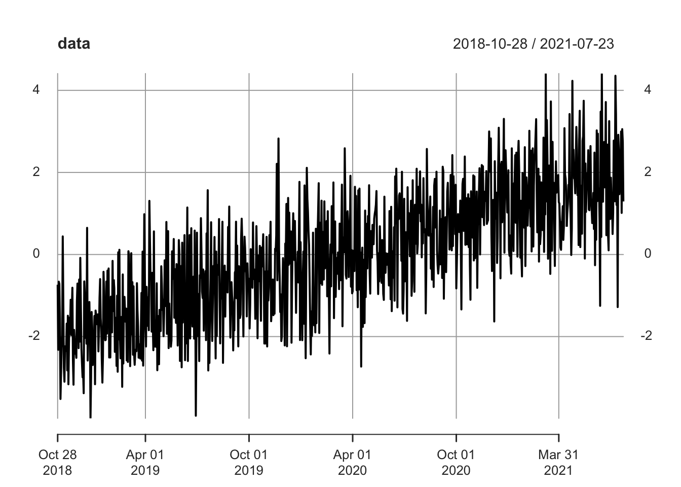

We can then use the roll_mean function to calculate, well, a rolling mean of this data! We can input how large we want out ‘window’ to be (is this a 30-day rolling mean? 40 day? etc.) with the width argument. Here, we will do a monthly, 30-day rolling mean. We could also use the weights argument to specify how we are going to weight the different data points, which we will show in a later example.

data_roll <- roll_mean(data, width = 30)
head(data_roll, 35)

##                 [,1]
## 2018-10-28        NA
## 2018-10-29        NA
## 2018-10-30        NA
## 2018-10-31        NA
## 2018-11-01        NA
## 2018-11-02        NA
## 2018-11-03        NA
## 2018-11-04        NA
## 2018-11-05        NA
## 2018-11-06        NA
## 2018-11-07        NA
## 2018-11-08        NA
## 2018-11-09        NA
## 2018-11-10        NA
## 2018-11-11        NA
## 2018-11-12        NA
## 2018-11-13        NA
## 2018-11-14        NA
## 2018-11-15        NA
## 2018-11-16        NA
## 2018-11-17        NA
## 2018-11-18        NA
## 2018-11-19        NA
## 2018-11-20        NA
## 2018-11-21        NA
## 2018-11-22        NA
## 2018-11-23        NA
## 2018-11-24        NA
## 2018-11-25        NA
## 2018-11-26 -1.920049
## 2018-11-27 -1.966005
## 2018-11-28 -1.969226
## 2018-11-29 -2.023997
## 2018-11-30 -2.084060
## 2018-12-01 -2.069656

plot(data_roll)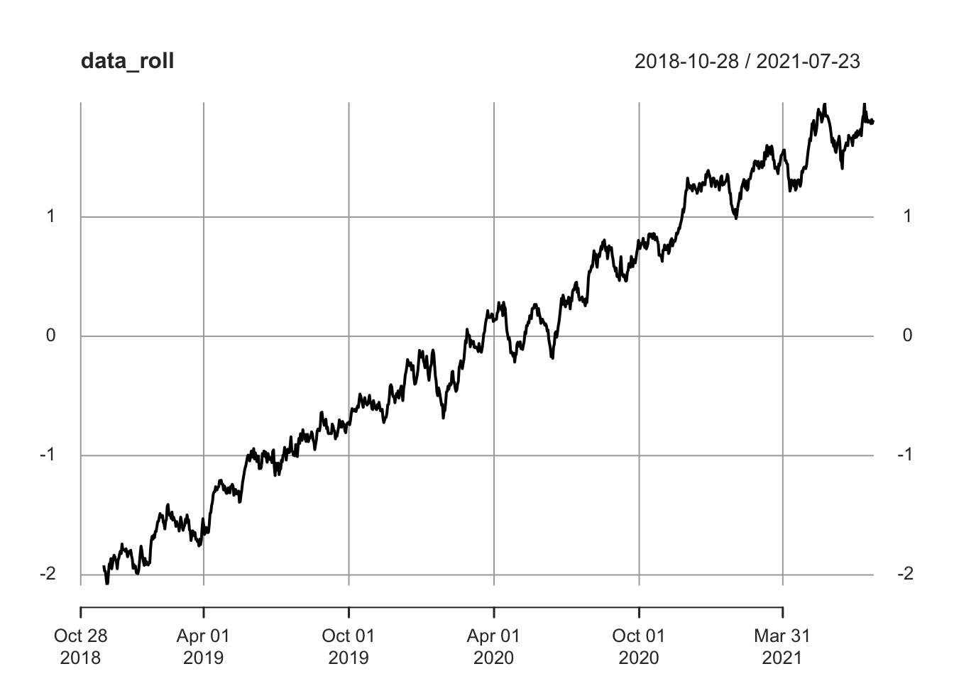

Note that data_roll is a time series, just like the data we fed into it. Also note that the first 29 values are NA because we are using a 30 day window (up to 29 days in, we don’t have 30 days with which to calculate a 30-day rolling mean!). Also note that we can easily plot the rolling mean, which gives us a much cleaner visual.

One benefit of the roll package is the speed; it’s significantly faster than some of the more conventional functions like rollapply (to read about why roll is so fast, just check the documentation by typing ?roll in your console; the discussion behind the processing speed is more applicable in a computer science book!). We can perform the same 30-day rolling mean with rollapply and roll_mean and see the speed difference for ourselves:

start <- Sys.time()
tail(rollapply(data, width = 30, FUN = mean))

##                [,1]
## 2021-07-18 1.794799
## 2021-07-19 1.803358
## 2021-07-20 1.782620
## 2021-07-21 1.817621
## 2021-07-22 1.785358
## 2021-07-23 1.812763

Sys.time() - start

## Time difference of 0.07307601 secs

start <- Sys.time()
tail(roll_mean(data, width = 30))

##                [,1]
## 2021-07-18 1.794799
## 2021-07-19 1.803358
## 2021-07-20 1.782620
## 2021-07-21 1.817621
## 2021-07-22 1.785358
## 2021-07-23 1.812763

Sys.time() - start

## Time difference of 0.004031897 secs

In addition to calculating means, the roll package uses a similar structure to calculate key statistics on both univariate and multivariate time series data. Some other useful functions include roll_max, roll_sum, roll_sd (standard deviation) and roll_lm (linear regression), just to name a few.

2.4 ggplot

The base R graphics package is reasonably versatile and useful, but the ggplot2 package provides access to a much more attractive, flexible suite of visuals.

Many R users don’t work with ggplot2 because it can be tricky to learn. The biggest barrier to entry is that ggplot2 likes data in the long format instead of the wide format. Here is an example of the ‘wide’ format, which you likely think of as the standard, default format:

# replicate
set.seed(0)

# initialize data
data <- matrix(round(rexp(10 * 5, 1 / 5), 1), 
               nrow = 10,
               ncol = 5)
data <- cbind(1:10, data)

# convert to data.table and name
data <- data.table(data)
names(data) <- c("day", "matt", "tom", "sam", "anne", "tony")

# view data
data

##     day matt  tom  sam anne tony
##  1:   1  0.9  3.8  3.2  0.2  5.1
##  2:   2  0.7  6.2  1.5  1.6  6.5
##  3:   3  0.7 22.1  2.8  6.6  6.3
##  4:   4  2.2  5.3  0.5  1.0  2.8
##  5:   5 14.5  5.2  0.3  5.1  1.5
##  6:   6  6.1  9.4  2.9  1.5  6.5
##  7:   7  2.7  3.3 19.8  3.6  5.0
##  8:   8  4.8  1.7  5.9  3.8  2.6
##  9:   9  0.7  2.9  5.0  1.2 10.0
## 10:  10  7.0 11.8  7.2  5.4  2.1

This data could represent, say, the total number of miles walked or run by five people over ten days (for example, Matt walked 2.7 miles on day 7). Note that each row in the data.table is a day, and each column is a person.

We can can convert the data to ‘long’ format using the melt function:

data_long <- melt(data, id.vars = "day")
head(data_long, 15)

##     day variable value
##  1:   1     matt   0.9
##  2:   2     matt   0.7
##  3:   3     matt   0.7
##  4:   4     matt   2.2
##  5:   5     matt  14.5
##  6:   6     matt   6.1
##  7:   7     matt   2.7
##  8:   8     matt   4.8
##  9:   9     matt   0.7
## 10:  10     matt   7.0
## 11:   1      tom   3.8
## 12:   2      tom   6.2
## 13:   3      tom  22.1
## 14:   4      tom   5.3
## 15:   5      tom   5.2

Note that we now have three simple columns in the data table: the ‘id’ column (which we specified in melt with the argument id.vars), the ‘variable’ column (which identifies which person that this specific row refers to) and the ‘value’ column (which identifies how far that person walked or ran on that day). This is considered ‘long’ data because every observation has its own row; that makes it pretty long!

While long data might seem unfamiliar, ggplot2 likes this format. We can think of making a ggplot2 chart as adding blocks on top of each other to make a picture (instead of drawing one picture all at once). For instance, we can always just start with a blank canvas with the ggplot function:

ggplot()

And we can add a title to this blank canvas by adding (with the + operator; this reinforces the idea that we are always adding pieces to a blank canvas) the ggtitle function:

ggplot() +
  ggtitle("First ggplot!")

Let’s try plotting our data_long. We usually put this right into our initial ggplot function and specify what our x and y values will be within the aes argument of ggplot (aes stands for aesthetics).

ggplot(data_long, aes(x = day, y = value)) +
  ggtitle("First ggplot!")

Hmm…we see a nice grid, but no data! We can add lines or points with the geom_line and geom_point functions. Let’s try points:

ggplot(data_long, aes(x = day, y = value)) +
  ggtitle("First ggplot!") +
  geom_point()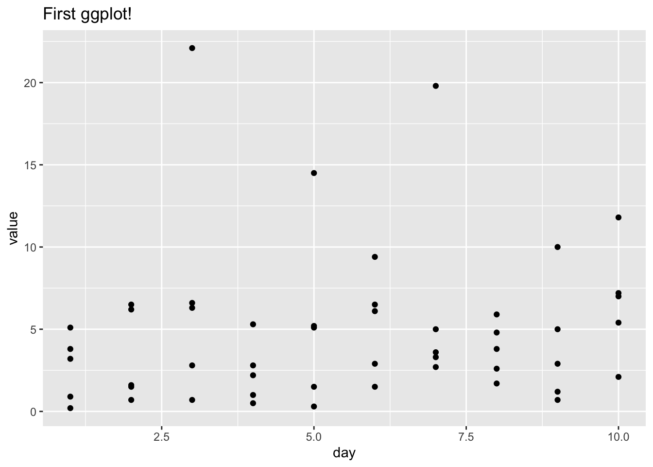

This still isn’t ideal because we can’t tell who is who (which points are Matt? Which points are Tom?). Luckily, we can specify how we want to color the points (here, by person) with the color parameter in aes. This is why it’s so nice to have data in the long format; each row as an x value, a y value and a ‘categorical’ value to tell us which group the observation is in!

ggplot(data_long, aes(x = day, y = value, color = variable)) +
  ggtitle("First ggplot!") +
  geom_point()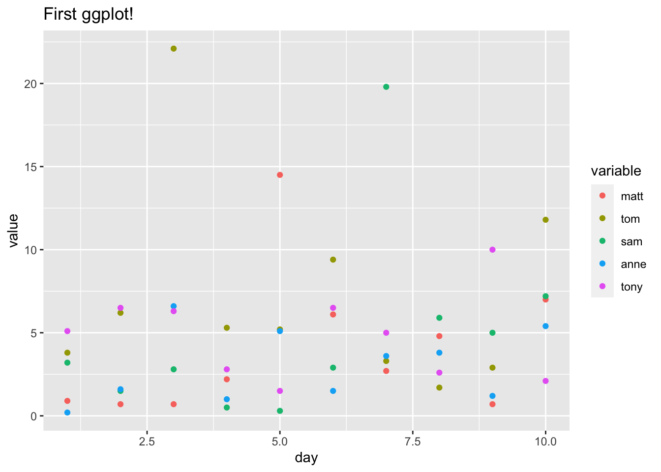

These are just the basics, but we can really make our chart ‘fancy’ by adding some simple functions: xlab and ylab give us the axis labels, the alpha argument in geom_line gives us the darkness of the line (0 to 1, 0 being invisible and 1 being full color), geom_smooth allows us to add smoothed trends for each line (and setting the se, or ‘standard error,’ argument in geom_smooth to FALSE removes the default shaded bands, which provide a sort of ‘confidence interval’ for the), geom_hline allows us to draw a horizontal line (hline stands for horizontal line; in the function, we specify the yintercept to be 0) and theme_bw adds a simple black and white theme (there are some really neat themes, including Wall Street Journal and 538, which you can find here).

ggplot(data_long, aes(x = day, y = value, color = variable)) +
  geom_line(alpha = 1 / 2) +
  ggtitle("First (fancy) ggplot!") + 
  geom_smooth(se = FALSE) +
  xlab("days") + ylab("miles traveled") +
  geom_hline(yintercept = 0) +
  theme_bw()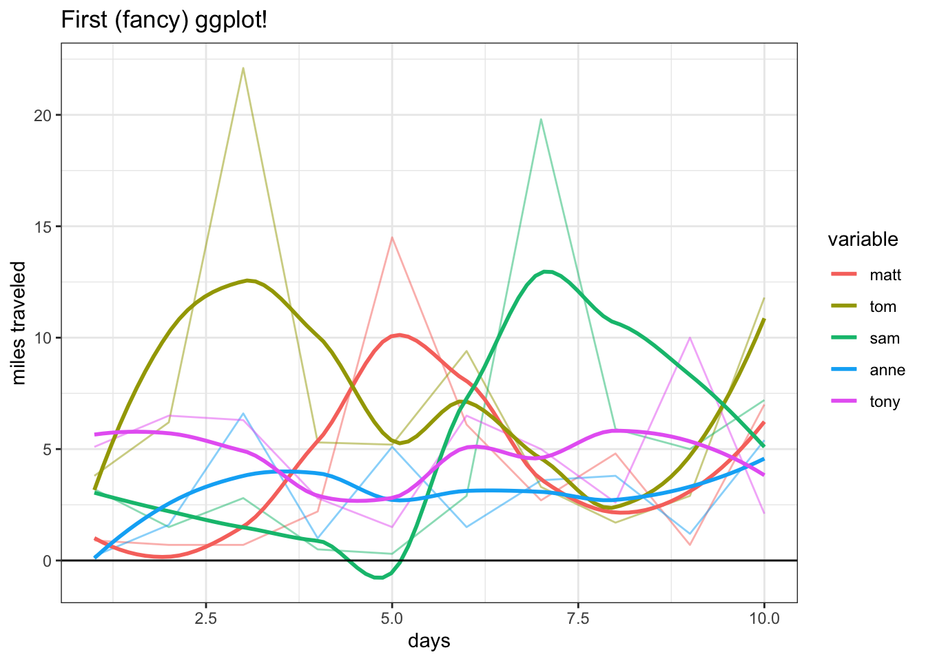

One last nifty tip is to use facet_wrap, which, instead of coloring each variable differently, creates a different chart for each variable (we could still color the lines differently with the col argument if we so desired):

ggplot(data_long, aes(x = day, y = value)) +
  facet_wrap(~variable) +
  geom_line(alpha = 1 / 2) +
  ggtitle("First (fancy) ggplot!") + 
  geom_smooth(se = FALSE) +
  xlab("days") + ylab("miles traveled") +
  geom_hline(yintercept = 0) +
  theme_bw()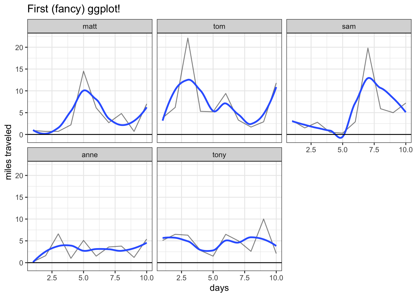

We simply put the variable we want to facet on (here, just variable) inside the facet_wrap function (don’t forget to add the ~ syntax!).

Note that, if we had even more categorical variables, we could facet by one variable and color by another variable; ggplot allows us to easily view complicated relationships and data breakdowns.

2.5 Optimizers (optim)

This is not a mathematics book and thus we won’t delve too deeply into the topic of optimization. However, we are hopefully all familiar with simple, single-variable optimization: we take a function $f(x)$ and find a value $x$ (often subject to some constraints) that minimizes (or maximizes) $f(x)$.

A commonly used function for optimization in R is optim. For example, say we define $f(x)$ such that:

\[f(x) = -(x - 1) ^ 2\]

We can define this function in R and even plot the output for a range of $x$ values:

# define function
FUN_negsqrt <- function(x) {
  return(-(x - 1) ^ 2)
}

# calculate output
x <- seq(from = -10, to = 10, by = 1)
y <- sapply(x, FUN_negsqrt)
data <- data.table(x = x, y = y)
ggplot(data, aes(x = x, y = y)) +
  geom_point() +
  xlab("x") + ylab("f(x)")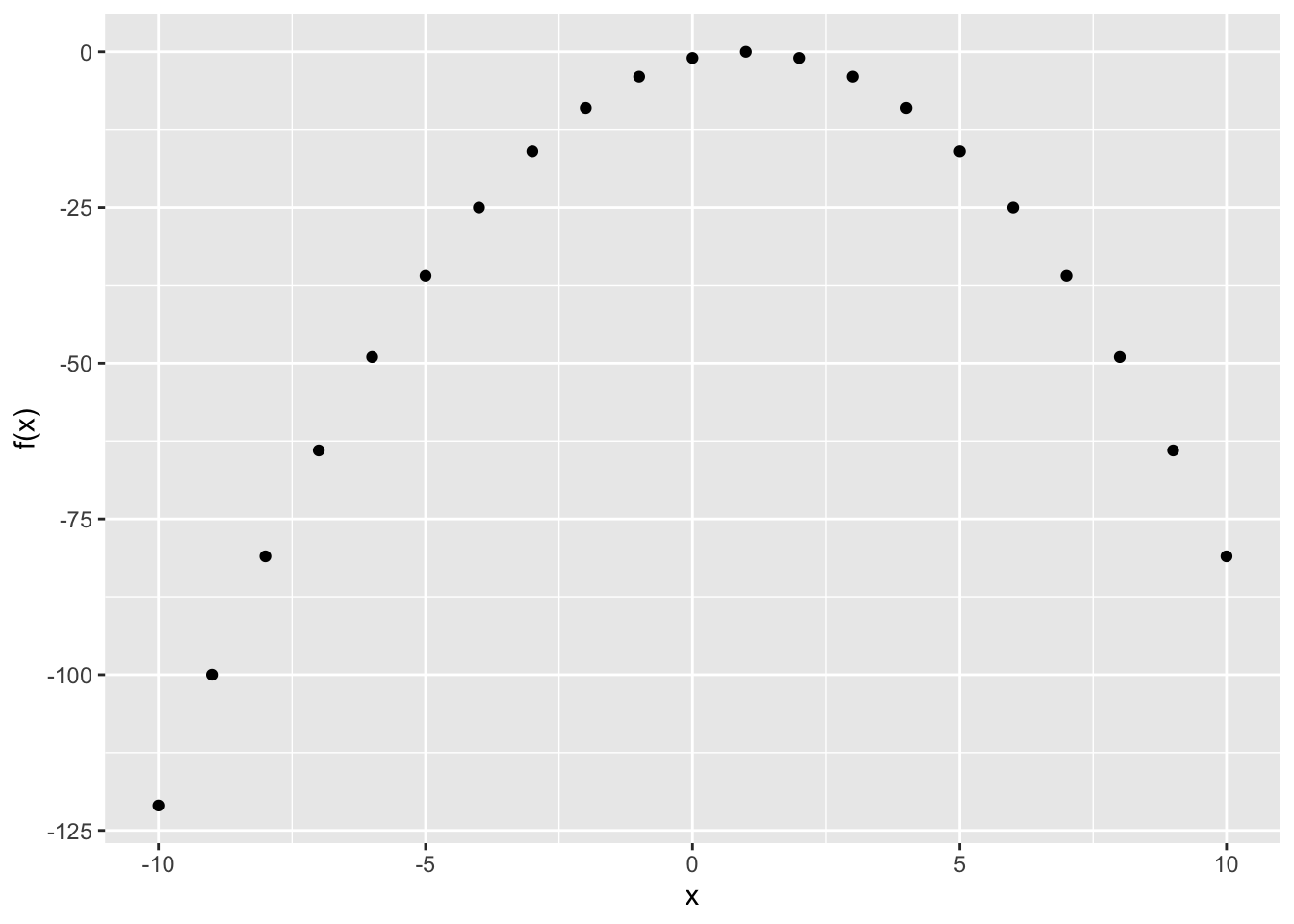

It is pretty clear that this function is maximized at $x = 1$ (the further we move from $x = 0$, the lower $f(x)$ seems to fall). We can even check this mathematically the ‘old school way’ with $f^{\prime}(0)$; that is, taking the derivative of $f(x)$ and plugging in 0. We can expand $-(x - 1)^2$:

\[-(x - 1)^2 = -x^2 + 2x - 1\]

Taking the derivative yields:

\[-2x + 2 - 1\]

And plugging in 0 for $x$ yields just $1$, which confirms our visual suspicions.

Given that this is a simple function for which we know the maximum point, this is a good candidate for testing the optim function in R. There are a couple of key arguments in this function that we need to be aware of:

fn: simply put, the function that we want to optimize! Here, we have defined it as FUN_negsqrt.
par: the initial value for the parameter we are optimizing (i.e., where the optimizer should start looking). We set it to 0 here, although, because this is a relatively simple function, the optimizer will likely find the solution no matter the starting spot!
lower and upper: the constraints for the parameter that we are optimizing (in our example above, the value $x$). In the below example, we set the upper bound to 10 and the lower bound to -10, essentially saying “find the maximum of $f(x)$ such that $|x| \leq 10$.” If we are using lower and upper, then we have to use the Brent method (set the method argument to Brent).
control: we can set this to list(fnscale = -1) if we want to maximize the function (optim minimizes by default). Of course, we could also just include an extra negative sign in the function instead!

# optimize
optim(fn = FUN_negsqrt, par = 0, control = list(fnscale = -1),
      lower = -10, upper = 10,
      method = "Brent")

## $par
## [1] 1
## 
## $value
## [1] -4.930381e-32
## 
## $counts
## function gradient 
##       NA       NA 
## 
## $convergence
## [1] 0
## 
## $message
## NULL

Let’s examine some of the crucial output. The $par value gives the result of the optimization; i.e., the value of $x$ that optimizes $f(x)$. We knew coming in that this value was $1$ and the output confirms it; optim works! The $value output gives the value of $f(x)$ when evaluated at $par, the optimal value; here, we can see that it is (extremely close) to zero (e-32 means $10^{-32}$). Finally, the $convergence output indicates if our optimizer successfully converged on a solution: this is 0 if we successfully converged and 1 if the iteration limit was reached (i.e., the optimizer looked too long, couldn’t find a solution and timed out). There are other less common potential values of $convergence, which you can investigate on the help page for the optim function (just type ?optim).

Just to confirm that the fnscale piece is doing what we think it’s doing, we can remove the control = list(fnscale = -1) (so that we minimize instead of maximize) and add a negative sign in the function; this gives the same result.

FUN_negsqrt <- function(x) {
  return(-1 * (-(x - 1) ^ 2))
}

optim(0, FUN_negsqrt,
      lower = -10, upper = 10,
      method = "Brent")

## $par
## [1] 1
## 
## $value
## [1] 4.930381e-32
## 
## $counts
## function gradient 
##       NA       NA 
## 
## $convergence
## [1] 0
## 
## $message
## NULL

2.6 Recursion

We’re used to iteration as a coding technique in R; for loops and applies iterate across a list / vector / other object, applying some function to each element. Recursion is a different technique; if you search recursion, Google will provide Did you mean: recursion, which of course brings you back to the same page.

It’s probably best to demonstrate recursion with an actual example. Let’s define a function that takes the factorial of an integer; first, we can use our tried and trusted iterative technique. Note that R has a perfectly usable factorial function already (and, if we were making our own function purely for speed and simplicity, would probably do prod(1:x), where prod just takes the product); we are just using the factorial as a simple, understandable case to demonstrate the difference between recursion and iteration.

# define function
FUN_factorial <- function(x) {
  
  result <- 1
  for (i in 1:x) {
    result <- result * i
  }
  
  result
}

# confirm function works
FUN_factorial(5)

## [1] 120

# check time
system.time(FUN_factorial(1000))

##    user  system elapsed 
##       0       0       0

Not bad! The function works well and is very speedy (we used Sys.time to measure how fast our code was earlier; here we are demonstrating another technique, system.time, which wraps around the code we want to measure and returns the amount of time elapsed).

Let’s now try to define the factorial function recursively:

# define function
FUN_factorial <- function(x) {
  
  # break condition
  if (x == 1) {
    return(1)
  }
  
  # recurse
  return(x * FUN_factorial(x - 1))
}

# confirm function works
FUN_factorial(5)

## [1] 120

# check time
system.time(FUN_factorial(1000))

##    user  system elapsed 
##   0.003   0.001   0.003

Let’s parse through how this code works. Note that (unless x = 1, which we will get to), FUN_factorial returns the input x times, well, FUN_factorial with x - 1 as an input. This is what makes the function recursive; it calls itself!

Let’s think about how this code works for the simple example of x = 3. The function returns 3 times FUN_factorial(2), and FUN_factorial(2) returns 2 times FUN_factorial(1). Now note that, for FUN_factorial(1), the ‘break condition’ is triggered (the break condition being x == 1 in the above code), the function just returns 1. Then, we work our way back out: at the bottom level of x = 1, we return 1, which then multiplies by the 2 and the 3 from the earlier steps. The calculation looks something like this:

Call FUN_factorial(3). This returns 3 * FUN_factorial(2).
FUN_factorial(2) returns 2 * FUN_factorial(1), so, combining this with first part, we have 3 * 2 * FUN_factorial(1).
FUN_factorial(1) returns 1 because of the break condition.
We multiply 1 by the 2 from Step 2, and we are left with 2.
We multiply 6 by the 3 from Step 1, and we are left with 6.

Essentially, we go down into the function (Steps 1 - 3) until we reach the break condition, and then we climb up out of the function (Steps 4 and 5), making all of the calculations that we set up on the way down (while waiting for the break condition).

Naturally, this list gets quite long when we have to go further to find the break condition (like with FUN_factorial(1000)), but this simple example gives us an idea how the recursion is working.

Finally, note that the time elapsed was larger for our recursive function than our iterative function. Because of all of the steps that have to be held in memory (on the way down), recursion can actually be slower and less efficient than iteration. We can see this effect even more drastically if we consider coding the Fibonacci sequence (remember, in this sequence each number is the sum of the previous two) with iterative and recursive techniques (note that, in our recursive function, we need two break conditions: if x == 1, just return 1, and if x < 1, return 0, since the sequence is defined for positive integers and we don’t want to get weird results for anything below 0).

# iterative function
FUN_fib <- function(x) {
  
  # initialize
  result <- c(1, 1)
  
  # sum
  for (i in 3:x) {
    result <- c(result, sum(tail(result, 2)))
  }
  
  return(tail(result, 1))
}

# time it
system.time(FUN_fib(25))

##    user  system elapsed 
##   0.006   0.000   0.006

FUN_fib <- function(x) {
  
  # break conditions
  if (x == 1) {
    return(1)
  }
  
  if (x < 1) {
    return(0)
  }
  
  return(FUN_fib(x - 1) + FUN_fib(x - 2))
}

# time it
system.time(FUN_fib(25))

##    user  system elapsed 
##   0.138   0.001   0.140

Note that the recursive function takes much longer than the iterative function in this case; making two calls to FUN_fib within FUN_fib simply branches out the calculation much more, and the function gets very slow for large inputs.

Ultimately, recursion can be a useful tool because it is more elegant and readable (which is evident in even our simple examples) but can be inefficient and slow because of the sheer amount of memory it uses.

2.7 Styling

We’ll close this chapter with a note on something crucial that many R users forgo: styling. This is essentially the ‘formatting’ of your code; i.e., how the code looks to the human reader. Two code chunks that produce the same result when executed can have different style; the code looks the same to the computer, but different to us!

For a full guide on standard style practices, see Hadley Wickham’s style guide. We will report and discuss some of the more crucial (and more common) aspects of style here.

When commenting your code, it’s important to include a space after the # so that the human reader can more easily read when the comment starts. It’s also important to keep your comments succinct and neat; if you have something verbose to say, simply say it in a text chunk like this one before your code chunk.

# good comment

#bad comment




# this is a good, succinct comment

# this is a bad comment because it 
# doesn't get to the point and
# takes up a big chunk of the page and also has an extra long line

One of the subtlest conventions in R is using <- for assignment instead of =. Many are annoyed by this tendency; what’s the difference? If anything, <- is an extra keystroke (even two extra keystrokes, because you have to hold down ‘shift’)!

There are some more advanced programming reasons for why <- is preferred (which you can read about here) but, as a practical user, we can keep these two key reasons in mind:

Using <-, which looks like an arrow pointing to the left, means that we will never forget that the direction of assignment is left to right (i.e., x <- 4 means ‘put the value 4 into x’ instead of ‘put the value x into 4’). Naturally, with an equals sign, this direction isn’t clear (you can also do rightwards assignment, or 4 -> x, although this is far, far less common). It sounds silly to think that we will need to be constantly reminded of the direction of assignment. However, when working with long, complicated code, it can be surprising how often really simple errors pop up. It can’t hurt to eliminate the risk of making an assignment error!
Using <- for assignment makes it far easier for a human reader to pick out different sections of the code. Since we don’t use = for assignment, if the reader is scanning the code and sees an equals sign, they can be more certain that they are looking at a function (since =, not <-, is used for the assignment of arguments in functions).

All told, don’t sweat that extra keystroke!

# good assignment
x <- 4

# bad assignment
x = 4

You can access the booleans (true or false in R) either with TRUE and FALSE or with T and F. It adds a few keystrokes, but just use the full name. It’s easier to read and, oddly, it is possible to assign values to T but not to TRUE (i.e., T <- 4 will execute but TRUE <- 4 throws an error; the same with FALSE and F), in which case, if you used T, you would be calling an object that is not a boolean!

# good boolean
TRUE; FALSE

## [1] TRUE

## [1] FALSE

# bad boolean
T <- 5
F <- "hi"
T; F

## [1] 5

## [1] "hi"

Space out your arithmetic; make sure that you have a space between each number and operator (i.e., +, -, *, /, ^, etc.). It makes it much easier to read!

# good arithmetic
6 * 5 - 4 ^ 2

## [1] 14

# bad arithmetic
6*5-4^2

## [1] 14

With loops and if statements, make sure that you have the proper spacing: include a space after for, if, etc., as well as after the closing parentheses. Again, the extra spacing makes reading easier.

# good loop
for (i in 1:10) {
  # do something
}


# bad loop
for(i in 1:10){
  # do something
}

# good if statement
if (2 + 2 != 4) {
  # do something
}

# bad if statement
if(2 + 2 != 4){
  # do something
}

When defining functions, make sure to use the same spacing structure as loops and if statements. Also, when naming functions, it’s useful to preface the name with FUN_ so that you automatically know the object is a function (instead of a vector, constant or some other object). Similarly, you’ll see that we often label any data with the prefix data_.

# good function
FUN_square <- function (x) {
  return(x ^ 2)
}

# bad function
square = function(x){
  return(x^2)
}