Chapter 3 Stochastic Properties

“Time is making fools of us again.” - Albus Dumbledore

Motivation

After a couple of introductory chapters, we can finally turn to the subject at hand. In this chapter, we will define stochastic processes and discuss some of their properties. We will also review a number of simple stochastic properties and use R to better understand their behavior.

3.1 Stochastic Definitions

It can be hard to define a subject in a single sentence. Think about it: how would you succinctly define ‘mathematics,’ or even ‘statistics?’ We are lucky that a ‘stochastic process’ has a simple, one line definition:

A random variable that changes through time

We’re cheating a bit by leaning on the definition of ‘random variable,’ but still, we have a simple, seven-word definition for an immensely complicated topic!

We denote random variables with capital letters like $X$. We denote stochastic random variables with $X_t$, which simply means ‘the value of $X$ at time $t$.’ We’ll start with potentially the simplest stochastic process: a Bernoulli Process.

\[X_t \sim Bern(p)\]

For $t = 1, 2, ...$ (this is called the index of the process), and all of the $X_t$ random variables are independent. This is a discrete stochastic process because the index is discrete; stochastic processes with continuous indices (continuous intervals of the real line) are considered continuous stochastic processes (this distinction is similar to the one we make with the supports of discrete and continuous random variables!).

Since we know that a Bernoulli is essentially a coin flip that takes on the value 1 with probability $p$ and takes on the value 0 with probability $1-p$, this stochastic process is just a series of zeroes and ones. For our starting stochastic process, let’s have $p = 1/2$.

# generate a Bernoulli process
data <- data.table(t = 1:100,
                   X = rbinom(100, 1, 1 / 2))

# visualize
ggplot(data, aes(x = t, y = X)) +
  geom_line() +
  theme_bw() +
  ggtitle("A Bernoulli Process") +
  ylim(c(-2, 2))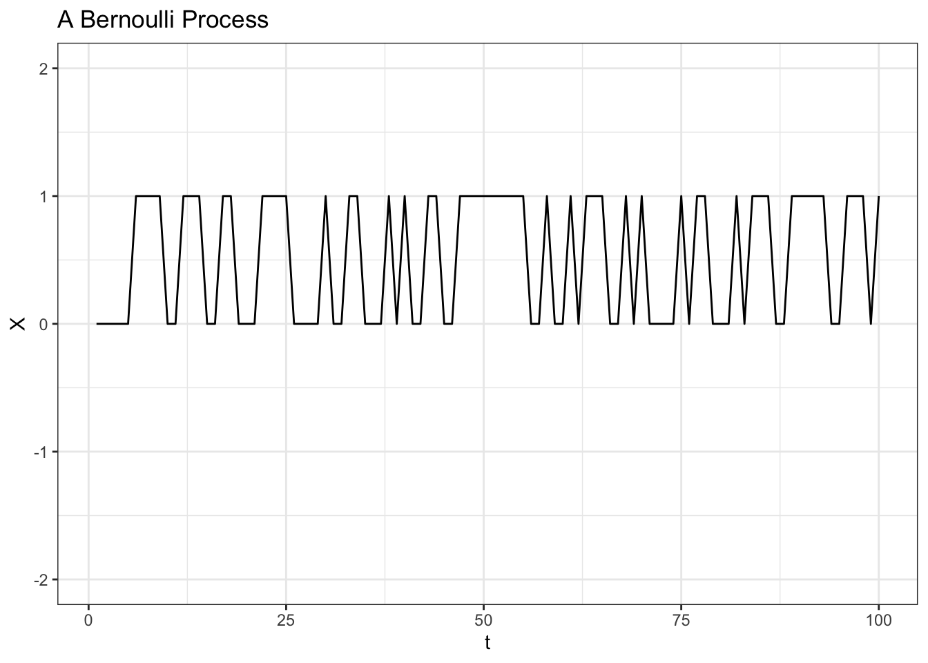

It’s important to remember that stochastic processes are still random variables. That is, $X_t$ (and $X_4$, $X_{17}$ and $X_{368}$, and all of the other steps in the process) has an expectation, a variance, moments, density functions, etc. In this specific case, for example, we have:

\[E(X_t) = \frac{1}{2}\]

\[Var(X_t) = \frac{1}{4}\]

\[P(X_t = 1) = P(X_t = 0) = \frac{1}{2}\]

For all values of $t$ in the index $\{1, 2, ...$}. Of course, this type of generality isn’t strictly necessary: we will be working with processes where we don’t have these neat solutions for all values of $t$ in the index (i.e., where the distribution of the process changes with $t$, in which case we might have $E(X_1) \neq E(X_2)$, or something along these lines).

3.2 Properties

The Bernoulli Process is exceedingly simple, so we will use it to explore some of the different properties of stochastic processes.

3.2.1 Stationarity

Colloquially, a stochastic process is strongly stationary if its random properties don’t change over time. A more rigorous definition is that the joint distribution of random variables at different points is invariant to time; this is a little wordy, but we can express it like this:

\[F_{t_1, t_2, ..., t_n} = F_{t_1 + k, t_2 + k, ..., t_n + k}\]

For all $k$, $n$ and sets of time intervals $t_1, t_2, ...$ in the stochastic process.

We introduced some new notation here; let’s make sure that we are familiar with all of the notation in the above equation. First, $F_{t_1}$ is the CDF (cumulative distribution function) of $X_{t_1}$, or the stochastic process at time $t_1$ (remember, we simply have that $F_{t} = P(X_{t} < x)$; this is the definition of a CDF). Then, $F_{t_1, t_2}$ is the joint CDF of $X_{t_1}$ and $X_{t_2}$, or $P(X_{t_1} < x_1, X_{t_2} < x_2)$. What this is equation is saying, then, is that a stochastic process is strongly stationary if the joint distribution of $X_t$ at times $t_1, t_2, ..., t_n$ is equal to the joint distribution of $X_t$ at times $t_1 + k, t_2 + k, ..., t_n + k$ (i.e., the time indices $t_1, t_2$ etc. shifted by $k$. For example, we might be asking ‘is the joint distribution of the stochastic process at time points 1 and 2 the same as the joint distribution of the stochastic process at time points 3 and 4?’).

Our Bernoulli Process is an i.i.d. process; that is, the different values of $X_t$ (at different time points $t$) are all independent and identically distributed Bernoulli random variables. Because the Bernoullis are independent, their joint CDF is just the product of the marginal CDFs:

\[F_{t_1, t_2, ..., t_n} = F_{t_1} \cdot F_{t_2} ... \cdot F_{t_n}\]

And, since the stochastic process has identical distributions $Bern(p)$ at every time point, we have:

\[F_{t_1} \cdot F_{t_2} ... \cdot F_{t_n} = F_{t_1 + k} \cdot F_{t_2 + k} ... \cdot F_{t_n + k}\]

So, the Bernoulli is strongly stationary! In fact, any i.i.d. process (because, by definition, the random variable has identical, independent distributions at different time point) is strongly stationary!

Weak stationarity, naturally, has less restrictive conditions than strong stationary. A stochastic process $X_t$ is weakly stationary if it meets these three conditions:

The mean of the process is constant. That is, $E(X_t) = \mu$ (where $\mu$ is some constant) for all values of $t$.
The second moment of $X_t$, or $E(X_t ^ 2)$, is finite.
We have:

\[Cov(X_{t_1}, X_{t_2}) = Cov(X_{t_1 - k}, X_{t_2 - k})\]

For all sets of $t_1, t_2$ and all values of $k$. That is, the covariance between two points only changes as the distance between them changes (i.e., $k$), not as we move along in time. That is, $Cov(X_5, X_8)$ must equal $Cov(X_{11}, X_{14})$ because $X_5$ is as far from $X_8$ as $X_{11}$ is from $X_{14}$ (three time points away).

We can quickly check if our Bernoulli Process is weakly stationary (we will again use $p$ as the parameter of the Bernoulli to keep the notation general):

$E(X_t) = p$, because each $X_t$ is i.i.d. $Bern(p)$. So, yes, the mean is constant through time!
Since $X_t ^ 2$ just takes on values 1 and 0, and these values don’t change when they are squared (1 goes to 1 and 0 goes to 0), we have $X_t ^ 2 = X_t$ and thus $E(X_t ^ 2) = E(X_t) = p$. Therefore, the second moment of $X_t$ is indeed finite (the maximum value of $p$ is $1$).
Finally, since the $X_t$ values are independent, we have that $Cov(X_j, X_k) = 0$ for all $j \neq k$.

So, a Bernoulli Process is weakly stationary!

That might have seemed like a lot of extra work. Didn’t we show that the Bernoulli Process was strongly stationary? Well, unfortunately, strong stationarity does not necessarily imply weak stationarity, and weak stationarity does not necessarily imply strong stationarity. Let’s see if we can construct counterexamples in both cases: something that is strongly stationary but not weakly stationary, and something that is weakly stationary but not strongly stationary.

Let’s define a new stochastic process $Y_t$ that takes on $X_t$ when $t$ is even and simply takes on the constant $1/2$ when $t$ is odd. We can simulate this easily in R (using the ‘modulo’ function $%%$ which gives us the remainder of one number divided into another number):

# replicate
set.seed(0)

# generate a Bernoulli process
data <- data.table(t = 1:100,
                   X = rbinom(100, 1, 1 / 2))

# generate Y
data$Y <- data$X
data$Y[data$t %% 2 == 1] <- 1 / 2

# visualize
ggplot(data, aes(x = t, y = Y)) +
  geom_line() +
  theme_bw() +
  ggtitle("Bernoulli Process at even time points, 1/2 at odd time points") +
  ylim(c(-2, 2))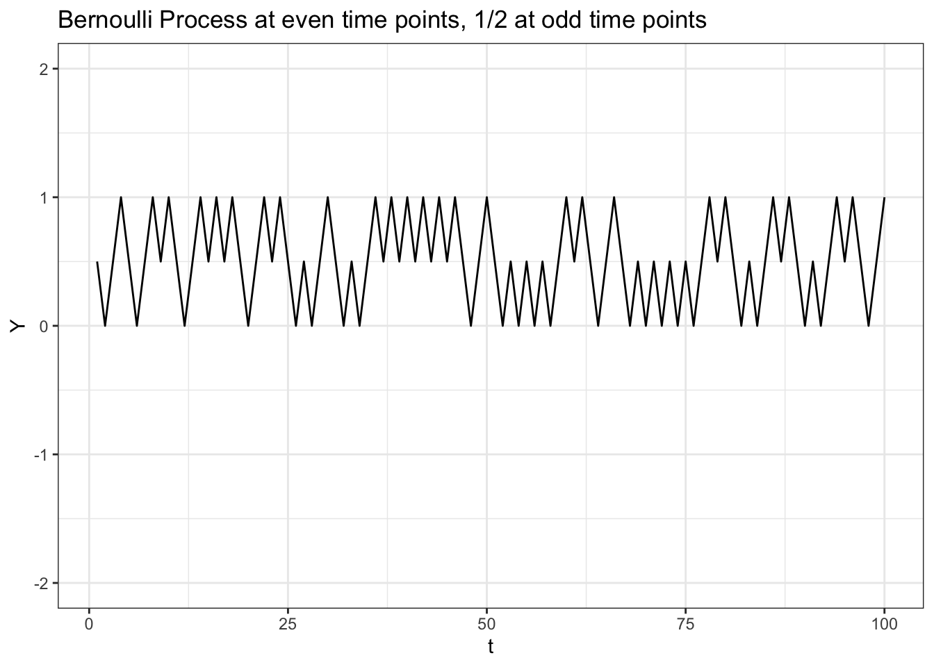

Let’s check to see if this process is weakly stationary by running through the three conditions.

$E(Y_t) = 1 / 2$, since, when $t$ is even, we have a $Bern(1/2)$, and when $t$ is odd, we simply have the value $1/2$.
When $t$ is even, we have a $Bern(1/2)$ random variable, and we have seen above that the second moment is finite (we just have that $p = 1/2$). When $t$ is odd, we have the constant $1/2$, and the second moment of a constant is just the constant squared ($1/4$). So, the second moment is finite.
Finally, since the $Y_t$ values are independent, we have that $Cov(Y_j, Y_k) = 0$ for all $j \neq k$.

So, $Y_t$ is indeed weakly stationary!

Now we can test for strong stationarity. We can check the simplest case:

\[F(Y_1) \stackrel{?}{=} F(Y_2)\]

We know that $Y_1$ is just a constant and that $Y_2 \sim Bern(1/2)$. These clearly have different CDFs (one quick intuitive check is that $Y_2$ has a non-zero probability of being above $1/2$ whereas $Y_1$ can only be $1/2$), so we can say:

\[F(Y_1) \neq F(Y_2)\]

Therefore, $Y_t$ is not strongly stationary; the distribution changes with time (half the time the stochastic process is a Bernoulli random variable and half the time it is a constant!).

How about the other direction: a process that is strongly stationary but not weakly stationary? The simplest example is a process $X_t$ where each value is an i.i.d. Cauchy distribution. We won’t review the Cauchy distribution here, but the key is its second moment is not finite (in general, this is a notoriously finicky distribution: the mean, variance and MGF, along with a couple of other key characteristics, are all undefined). Therefore, $X_t$ is strongly stationary (it is an i.i.d. process), but it is not weakly stationary (the second moment is not finite, so one of the three criteria fails!).

3.2.2 Martingales

Colloquially, a stochastic process is a martingale if ‘we expect the next step to be right where we are.’

Mathematically, we say that a stochastic process $X_t$ is a martingale if:

\[E(X_{n + 1} | X_1, ..., X_n) = X_n\]

For any time $n$. We also require that $E(|X_n|)$ is finite.

So, at any time $n$, a stochastic process is a martingale if, conditioning on the entire observed history of the stochastic process up to time $n$ (this is often called the filtration), the expected value of the next step $X_{n + 1}$ is just $X_n$ (which has already been observed, since we are at time $n$).

Is our Bernoulli Process a martingale? Well, since each step is independent, we have:

\[E(X_{n + 1} | X_1, ..., X_n) = E(X_{n + 1})\]

And since $X_{n + 1} \sim Bern(1/2)$ like all of the other steps, we have:

\[E(X_{n + 1}) = 1/2\]

However, we know that $X_n$ will either be $0$ or $1$, so we can say:

\[E(X_{n + 1} | X_1, ..., X_n) \neq X_n\]

And therefore our Bernoulli Process is not a martingale.

Can we construct a simple stochastic process that is a martingale? Let’s try defining $Y_t$, where:

\[Y_0 = 0\] \[Y_t = Y_{t - 1} + \epsilon_t\]

Where $t = 1, 2, ...$ and $\epsilon_t$ is a series of i.i.d. $N(0, 1)$ random variables (standard normal random variables).

This is called a Gaussian Random Walk. The Gaussian part means ‘Normal’ and the Random Walk part means that, well, the process looks like it’s randomly walking around! We can easily simulate this process in R:

# replicate
set.seed(0)

# generate a Gaussian Random Walk
data <- data.table(t = 1:100,
                   Y = cumsum(rnorm(100)))

# visualize
ggplot(data, aes(x = t, y = Y)) +
  geom_line() +
  theme_bw() +
  geom_hline(yintercept = 0) + 
  ggtitle("Martingale?")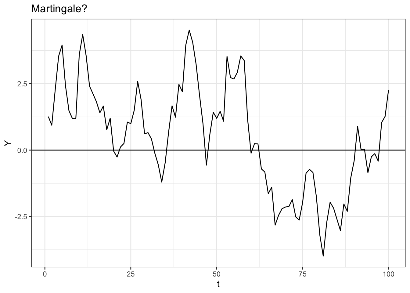

Let’s try to calculate the expectation of $Y_{n+ 1}$ given the history of $Y$ up to time $n$. We have:

\[E(Y_{n + 1} | Y_1, ..., Y_n) = E(Y_{n + 1} | Y_n)\]

Because $Y_{n + 1}$ is conditionally independent on $Y_1, Y_2, ..., Y_{n - 1}$ given $Y_n$ (i.e., if we know the value of $Y_n$, it doesn’t matter how we got there).

We can plug in for $Y_{n + 1}$:

\[E(Y_n + \epsilon_n | Y_n) = Y_n\]

Because $\epsilon_n \sim N(0, 1)$ and the expected value of $Y_n$ given $Y_n$ is, well, $Y_n$ (the ‘finite expectation’ piece is also satisfied; we know that $E(Y_n) = 0$, because $Y_n$ is essentially the sum of many standard normal random variables, each of which has expectation 0).

Therefore, $Y_t$ is a martingale, because the expected value of the next step is the step that we are currently at (conditioning on the history of $Y_t$ up to the current moment). Intuitively, this is because at each step we add something ($\epsilon_t$) with a mean of zero, so the expected value of the next time point in the series doesn’t move from where we are now (we are adding zero)!

3.2.2.1 The Shakespeare Problem

Martingales may seem pretty boring at first, but they allow us to solve pretty interesting problems. You’ve likely heard this before:

If you let a monkey bang on a keyboard long enough, it will write Shakespeare

We can use martingales to think about just how long this monkey will have to be ‘typing.’

Let’s make a couple of assumptions. The monkey types one letter at a time (come to think of it, is it possible to type more than one letter at a time?), and chooses each letter with equal probabilities ($1/26$ for each). Punctuation / cases (uppercase vs. lowercase) are irrelevant here.

Let $T$ be the random variable that gives the number of keys that the monkey presses until he types $OTHELLO$ (of King Othello fame). Find $E(T)$.

This can definitely be a tricky problem. We know that $E(T)$ is definitely pretty large (the monkey has to get seven letters in a row correct), but it can be challenging knowing where to start with this problem: there are some nasty hidden traps! For example, consider how, if the monkey successfully types $OTHE$, he can either type the next correct letter $L$, or he can type an incorrect letter. However, not all incorrect letters are created equal. If he types a non-$O$, he has to start over; however, if he types $O$, he lost his $OTHE$ progress but at least still has made on letter of progress (the $O$). This changes after the monkey has typed $OTHELL$; after this, all incorrect letters are created equal. Either the monkey types $O$ and ends the game, or types a non-$O$ and starts from scratch, which is different from what we saw above. These minor differences can quickly balloon into a nightmare if we try to solve the problem with a variety of conventional methods.

Instead, then, we’re going to use two tools to solve this problem. The first will be setting up a series of gamblers (yes, gamblers) that bet on the success of the monkey. Before the monkey hits each new letter, a new gambler enters the game and ponies up $\$1$. Let’s think about the first gambler (who bets on the monkey’s first letter): he puts up $\$1$ and gets $\$26$ back if the monkey hits $O$ (the first letter in $OTHELLO$) including his original $\$1$ (for a $\$25$ profit). If the monkey hits any other letter than $O$, the gambler loses his dollar. In this way, it’s a fair bet: the gambler has a $1/26$ probability of getting $26$ times his investment, and a $25/26$ probability of losing everything (the gambler profits $\$25$ with probability $1/26$ and loses his $\$1$ with probability $25/26$, so his expected profit is $25 \cdot (1 / 26) - 1 \cdot (25 / 26) = 0$).

A new gambler comes in before the monkey hits each letter. For example, if the monkey hits $K$ on the first letter, the first gambler loses his dollar and goes home, and a new gambler arrives and puts a dollar on the monkey hitting $O$ on the second letter.

It gets interesting if the monkey hits $O$. The active gambler gets $\$26$, and now bets all $\$26$ on the monkey hitting $T$ on the next letter with the same odds: if the monkey hits $T$, the gambler now has $26^2$ dollars, and if the monkey doesn’t hit $T$, the gambler loses everything. Again, this is a fair bet; the gambler has a $1/26$ probability of profiting $26^2 - 26$ (the $26^2$ dollars he gets back minus his original $26$ dollars) and a $25/26$ probability of losing his $26$ dollars. Therefore, his expected profit is still $0$:

\[(1 / 26) \cdot (26 ^ 2 - 26) - (25 / 26) \cdot 26 = 0\]

In addition to the gambler who won on the $O$ and now puts all of his $26$ dollars on $T$ coming next, a new gambler enters the game and puts one dollar on $O$ being struck next (i.e., the monkey starts typing $OTHELLO$ with the next letter). If $O$ is hit, the first gambler loses his $26$ dollars and the second gambler now has $26$ dollars and proceeds in the same way.

This sounds like a convoluted setup, but, amazingly, it will make our problem easier. Let us now define $M_n$ as the total winnings of all gamblers up to time $n$. We know that $M_n$ is a martingale; if, for instance, the monkey has hit ten non-$O$’s in a row, then we have $M_{10} = -10$ (10 gamblers have each lost a single dollar). Conditioning on $M_{10} = -10$ (really, conditioning on the history of the process up to time $10$, although $M_{10}$ is the only point we need here), our expected value for $M_{11}$ is, well, just $-10$. That’s because the new gambler who enters the game at the $11^{th}$ letter is making a fair bet; his expected profits are zero, so our expectation for the new total of all of the gamblers winnings is just the last value in the series (the $-10$ plus the expected zero dollars from this new gambler).

We can now unveil our second tool, which is Doob’s Optional Stopping Theorem. This states that, for a martingale $X_t$ with a ‘stopping time’ $\tau$ (the stopping time is just when we ‘stop’ the process) under certain general conditions ($X_t$ is bounded, or $T$ is bounded, or $E(T) < \infty$), we have that:

\[E(X_0) = E(X_{\tau})\]

That is, the expected value of the process at the stopping time is the same as the expected value of the process at the beginning!

We know that $M_t$ is a martingale, and $T$ is a stopping time (we stop once we hit $OTHELLO$), so we can apply Doob’s to this problem (we won’t do a formal proof for conditions, but consider why $E(T)$ might be finite). We know, then, that:

\[E(M_0) = E(M_T)\]

We know that $E(M_0)$ is just, well, zero, because this is the number of winnings before any of the gamblers have actually gambled! We thus have:

\[E(M_0) = 0 = E(M_T)\]

Let’s now think about $E(M_T)$. We know that, at time $T$, just after $OTHELLO$ has been hit, $T$ gamblers have put up one dollar, so there is a $-T$ term in this expectation. We also know that one (very lucky) gambler has won $26^7$ dollars (he won each bet that he put on) and (this is the tricky part), one gambler has won $26$ dollars (the gambler that bet on a $O$ when the monkey hit the last $O$ in Othello!). Therefore, we simply have:

\[0 = E(26^7 + 26 - T)\] \[0 = 26^7 + 26 - E(T)\] \[E(T) = 26^7 + 26\]

Incredible! We were able to solve this very tricky problem by setting up an (admittedly convoluted) gambling scheme and using a cool property of martingales; what’s more, the solution is broken into easily digestible parts!

3.2.3 Joint Stochastic Processes

As in most statistical fields, stochastic processes can be ‘levered up’ from the marginal (single process) to the joint (multiple processes). We will see a couple of examples of joint stochastic processes later on, so we can introduce some examples here and explore some of their key properties.

Let’s return to our Gaussian Random Walk:

\[Y_0 = 0\] \[Y_t = Y_{t - 1} + \epsilon_t\]

Where $t = 1, 2, ...$ and $\epsilon_t$ is a series of i.i.d. $N(0, 1)$ random variables.

Let’s now define a process $Z_t$:

\[Z_0 = 0\] \[Z_t = Y_t - \gamma_t\]

Where $t = 1, 2, ...$ and $\gamma_t$ is a series of i.i.d. $Expo(1)$ random variables.

We can easily visualize a simulation of these two processes:

# generate the processes
data <- data.table(t = 1:100,
                   Y = cumsum(rnorm(100)))
data$Z <- data$Y - rexp(100, rate = 1)

# visualize
ggplot(data, aes(x = t, y = Y)) +
  geom_line(col = "black") +
  geom_line(data = data, aes(x = t, y = Z), col = "red") +
  theme_bw() +
  geom_hline(yintercept = 0) + 
  ggtitle("Joint Processes Y (black) and Z (red)") +
  ylab("")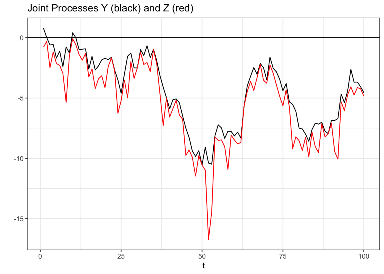

Now is a good time to introduce the concept of independence as it relates to stochastic processes. We say that two stochastic processes $X_t$ and $Y_t$ are independent if, for any sequence $(t_k, t_{k + 1}, ..., t_{k + n})$ where $k, n$ are positive integers less than $\infty$, we have that the vector:

\[\Big(X_{t_k}, X_{t_{k + 1}}, ..., X_{t_{k + n}}\Big)\]

…is independent of the vector…

\[\Big(Y_{t_k}, Y_{t_{k + 1}}, ..., Y_{t_{k + n}}\Big)\]

Colloquially, for $X_t$ and $Y_t$ to be independent, we must have that any subset of $X_t$ is independent to the same subset (on the same time points) of $Y_t$.

What does it mean for two vectors to be independent? To really get into the weeds here we would need some measure theory, which is beyond the scope of this book. We can think of this in our parlance; the random vector for $X_t$ above has joint density:

\[f_{x_t}(x_{t_k}, x_{t_{k + 1}}, ..., x_{t_{k + n}})\]

Where $f_{x_t}$ is just defined as the joint density of $X_t$ (note that if each $X_t$ was i.i.d., we would have that $f_{x_t}$ is just the product of the marginal densities of $X_t$ at all of the individual time points). Similarly, we have the joint density of $Y_t$:

\[f_{y_t}(y_{t_k}, y_{t_{k + 1}}, ..., y_{t_{k + n}})\]

And, similar to independence with marginal random variables, we can say that the vectors are independence if the joint density of both vectors $f_{x_t, y_t}$ is equal to the product of $f_{x_t}$ and $f_{y_t}$:

\[f_{x_t, y_t}(x_{t_k}, x_{t_{k + 1}}, ..., x_{t_{k + n}}, y_{t_k}, y_{t_{k + 1}}, ..., y_{t_{k + n}}) = f_{x_t}(x_{t_k}, x_{t_{k + 1}}, ..., x_{t_{k + n}}) \cdot f_{y_t}(y_{t_k}, y_{t_{k + 1}}, ..., y_{t_{k + n}})\]

That’s certainly a mouthful! Let’s return to our example of $Y_t$, the Gaussian Random Walk, and $Z_t$ above. We can test a very simple case; is the joint density of $Y_1$ and $Z_1$ equal to the product of the marginal densities of $Y_1$ and $Z_1$?

\[f(y_1, z_1) \stackrel{?}{=} f(y_1) f(z_1)\]

Immediately, we can see this is not the case; $Z_1$ can only be, at maximum, $Y_1$. The density of $Z_1$ is only defined up to $Y_1$, and thus we can’t multiply the marginal densities to get the joint densities. $Z_1$ and $Y_1$ are not independent, which means, by extension, $Z_t$ and $Y_t$ are not independent.

This example may seem excessively simple, but the concept of independence is important in stochastic processes.

3.2.4 Markov Property

Colloquially, a stochastic process with the Markov property only cares about its most recent state.

Mathematically, the stochastic process $X_t$ satisfies the Markov property if:

\[P(X_t|X_1, X_2, ..., X_{t - 1}) = P(X_t | X_{t - 1})\]

That is, within the filtration of $X_t$ (all of the information before time $t$), $X_{t - 1}$ tells us all the information that we need to know about $X_t$ (put another way, $X_t$ is conditionally independent of $X_1, X_2, ..., X_{t - 2}$ given $X_{t - 1}$).

Our Bernoulli Process is clearly Markov, since each step is just an i.i.d. Bernoulli, and thus:

\[P(X_t|X_1, X_2, ..., X_{t - 1}) = P(X_t | X_{t - 1}) = P(X_t)\]

That is, conditioning on the past doesn’t even tell us anything, because each step is independent of previous steps.

We can also consider our Gaussian Random Walk:

\[Y_0 = 0\] \[Y_t = Y_{t - 1} + \epsilon_t\]

Where $\epsilon_t$ is a series of i.i.d. $N(0, 1)$.

This is also Markov; given $Y_{t - 1}$, we have all of the information about $Y_t$ that we could get from the history the process; the only random part remaining is $\epsilon_t$, which is independent of $Y_t$.

3.2.5 Reflective Property

We can now turn to a fun property of certain stochastic processes. The reflective property invokes symmetry and yields a pretty neat result; we will be dealing with the reflective process for continuous stochastic processes.

Let $X_t$ be a continuous stochastic process such that, for all $t$ and $k < t$, we have that $X_t - X_{t - k}$ is a symmetric random variable about 0 (a random variable $Y$ is symmetric about 0 if $Y$ has the same distribution as $-Y$). That is, the increment of our process (amount that we add to our process over every interval) is symmetric.

To explore this property, we will introduce a new stochastic process: Brownian Motion. This is a stochastic process with a relatively simple structure but many applications. Let $X_t$ be Brownian Motion; we have that $X_0 = 0$ and:

\[X_t \sim N(0, t)\]

Remember that this is a continuous process, so the index is simply $t \geq 0$ (that is, the positive part of the real line). Brownian motion has some key characteristics; first, increments of Brownian motion are themselves Normal random variables. For example, where $s < t$, we have:

\[X_t - X_s \sim N(0, t - s)\]

This is intuitive; there is $t - s$ time from time $s$ to time $t$, so we have a Brownian motion with variance $t - s$ (this also explains why $X_t \sim N(0, t)$, because $X_t$ is essentially $X_t - X_0$, and $X_0$ is the constant 0). Now imagine another increment $X_w - X_v$ that is non-overlapping (that is, either $w$ and $v$ are both greater than $t$ or both $w$ and $v$ are both less than $s$, the point being that $w$ and $v$ aren’t in the interval between $s$ and $t$). We have that $X_w - X_v$ is independent of $X_t - X_s$. Naturally, if the intervals were overlapping, the two would be dependent.

We can clearly see that this is symmetric, by the definition of a Brownian Motion; as we stated above, the increments have a Normal distribution with mean 0, which is symmetric about 0.

Let’s generate a sample path of Brownian Motion to illustrate what the reflective property is.

Note that the way we generate Brownian Motion is similar to how we generate the Gaussian Random Walk; the difference is that, theoretically, the Brownian Motion is defined at every point on $t \geq 0$, and the Gaussian Random Walk is only defined on zero and positive integers. In our simulation, of course, we can’t quite get to the continuous $t \geq 0$, so we simply try to include more points in the same discrete interval. The result, in essence, is that we get closer to the continuous case.

We’ll be using, then, increments of $.01$ (we used increments of $1$ in the Gaussian Random Walk case). It’s important to get the standard deviation in our rnorm call correct: remember that the variance of each interval of a Brownian Motion is simply the distance in time stamps. Therefore, we want a variance of $.01$ and thus use sqrt(.01) for the standard deviation argument in rnorm (remember that the standard deviation is the square root of variance!).

# replicate
set.seed(0)

# generate a Gaussian Random Walk
data <- data.table(t = c(0, seq(from = .01, to = 10, by = .01)),
                   X = c(0, cumsum(rnorm(1000, mean = 0, sd = sqrt(.01)))))


# visualize
ggplot(data, aes(x = t, y = X)) +
  geom_line() +
  geom_hline(yintercept = 0) + 
  theme_bw() + ylab("") +
  ggtitle("Brownian Motion")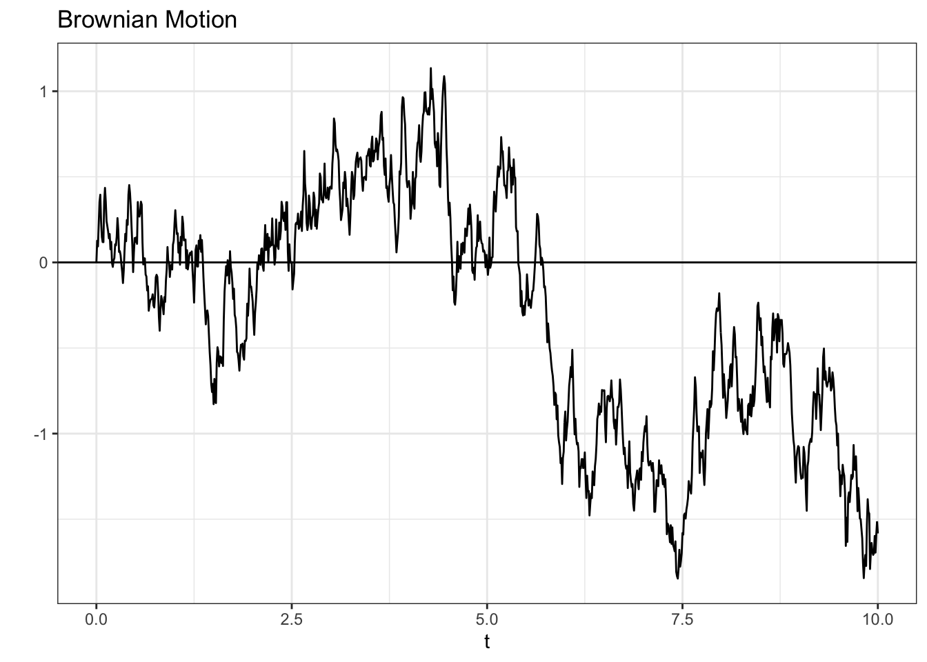

Here’s a video review of this stochastic process:

Click here to watch this video in your browser

Let us now see how we can use the reflective property to solve interesting problems relating to Brownian Motion.

# replicate
set.seed(0)

# generate a Gaussian Random Walk
data <- data.table(t = c(0, seq(from = .01, to = 10, by = .01)),
                   X = c(0, cumsum(rnorm(1000, mean = 0, sd = sqrt(.01)))))


# reflect
data$Y <- c(data$X[1], diff(data$X))
data$Y[(which(data$X > 1)[1] + 1):nrow(data)] <- -data$Y[(which(data$X > 1)[1] + 1):nrow(data)]
data$Y <- cumsum(data$Y)

# visualize
ggplot(data, aes(x = t, y = X)) +
  geom_line(col = "black") +
  geom_line(data = data, aes(x = t, y = Y), col = "red") +
  geom_hline(yintercept = data$X[which(data$X > 1)[1]], linetype = "dotted") +
  theme_bw() +
  geom_hline(yintercept = 0) + 
  ylab("") +
  ggtitle("Reflective Property")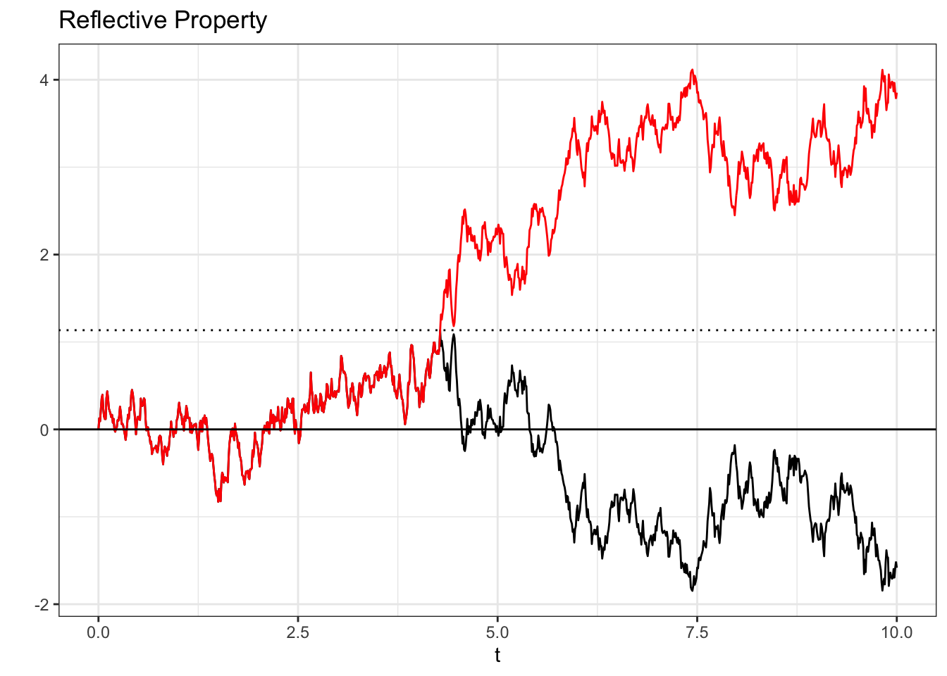

In this chart, we take a Brownian Motion (black line) and, the first time that this random walk breaches 1 (in this specific example, it hits $1.13$ at $t = 4.28$; remember that we can’t fully simulate the continuous case so we are just using an interval with smaller segments of length .01), we reflect the process about itself (about the line $1.13$, here; in the code above, you can see how we flip the increments of Y after X breaches $1$). The red line is, intuitively, this reflection (we could also simply reflect the process from the start about 0, instead of waiting for the process to hit some value).

Now, the reflection principle states that the black line has the same probability of being realized as the red line. That is, at time $t = 0$, these two paths have the same probability of occurring. For a proof here, we can rely on symmetry: since the increment at every time step is symmetric about zero and we are simply flipping all of the increments after a certain point to get from the black line to the red line, the two paths should have the same probability (remember, for a symmetric random variable $Z$, we have that $Z$ has the same distribution as $-Z$).

This may sound like a convoluted and useless property, but we can use it to solve some pretty interesting problems. For example, consider this question for $X_t$, our Brownian Motion above:

What is the probability that, by time $t = 100$, we have $max(X_1, X_2, ..., X_{100}) > 5$ but $X_{100} < 0$? More colloquially, what is the probability that $X_t$ hits a max above 5 but still ends below zero by time $t = 100$?

This seems like a challenging problem. There are a lot of ways that this condition could be achieved; theoretically, $X_t$ could breach 5 at any time (before $t = 100$) and fall from there (although, of course, this becomes less likely if there is less time to fall!). One first reaction might be to try to integrate across the whole timespan; we could potentially find the probability that $X_t$ breaches 5 by any point, and then the probability that, from that point, $X_t$ falls back below 0 by the time $t = 100$.

However, we can use the reflective property to make this problem far easier. Let us imagine a process that hits the 5, and then let us reflect that process about 5 for the rest of the period. As we saw above, these two paths have the same probability of occurring.

Now, we know that if the reflected path climbs above 10, then the original path has climbed below 0 (remember, we began to reflect the path as soon as the original path hit 5). Therefore, we simply need the probability that the Brownian motion ends above 10, or $P(X_{100} \geq 10)$. Since we have, by definition, that $X_{100} \sim N(0, 100)$, this becomes a simple calculation:

\[1 - \Phi\Big(\frac{10 - 0}{\sqrt{100}}\Big) = 1 - \Phi(\frac{1}{10})\]

Where $\Phi$ is the CDF of a standard Normal random variable. In R, we get:

1 - pnorm(10 / 10)

## [1] 0.1586553

We can simulate many paths of this Brownian motion to see if our answer makes sense (we will use intervals of .1 in our simulation):

# replicate
set.seed(0)
nsims <- 1000


# generate the Brownian motions
data <- replicate(cumsum(rnorm(1000, mean = 0, sd = sqrt(.1))), n = nsims)

# count how many paths hit 5 and ended below 0
results <- apply(data, 2, function(x) {
              if (max(x) >= 5 & tail(x, 1) < 0) {
                return(1)
              }
              
              return(0)
            })

mean(results)

## [1] 0.145

It looks like our empirical result is close to the analytical result we solved! You can try running more simulations (increasing nsims) to ensure that the probabilities match.

What started as a complicated problem, then, reduced drastically in complexity when we applied the reflective property; in general, the beauty of symmetry can reduce many difficult problems to smaller, much easier problems!

If you are still confused, this video may help to clear things up:

Click here to watch this video in your browser