Chapter 6 Kalman Filters

“I can see clearly now the rain is gone” -Johnny Nash

Motivation

Kalman Filters are not a new topic in Statistics, but nonetheless remain quite relevant: the potential uses for this tool widely vary. The crux of the Kalman Filter is to estimate the value of some ‘unknown state’ based on some observed data. Kalman Filters are built upon Stochastic Processes, and this chapter is thus a viable opportunity for us to explore a practical application of our subject.

6.1 Introducing Kalman Filters

We began to introduce what a Kalman filter is above: a tool that estimates an unknown state based on observed data (so that our estimation is a combination of this observed data and a prediction).

One intuitive example is estimating the location of a satellite orbiting Earth. We take the ‘unknown state’ to be the true, exact position of the satellite, which we are trying to estimate from the ground. First, we have a ‘prediction step’: we make a prediction about where the satellite will be in the future based on where it was launched and using knowledge about gravity, the Earth’s rotation, etc. Second, we have a ‘measurement step’: we have a sensor on the satellite that beams us back information about the satellite’s location (the information isn’t exactly perfect; if it was, we wouldn’t need to estimate the satellite’s location in the first place!), and we use this measurement to update our estimate of where the satellite truly is (again, it’s only an estimate because both our measurement and our prediction are noisy).

This is some simple intuition, but opens up a world of complexity: the unknown state, prediction and measurement can all have multiple dimensions (depending on the structure of the problem; what if, for example, we wanted the location of two satellites?). We can use Kalman Filters to rigorously define a useful approach to making these estimates.

As we will see, Kalman Filters assume Gaussian (Normally distributed) inputs. One convenient result of this is that Gaussian predictions, combined with Gaussian measurements, give Gaussian estimates. This links nicely into the next step of the Kalman Filter; if we make a Gaussian estimate at time $t$, we can feed that Gaussian estimate into the Kalman Filter to get another Gaussian estimate at time $t + 1$, and so on.

Finally, we will be orienting our discussion in a statistical sense, using Stochastic Processes, statistical distributions and the like to frame the Kalman Filter (traditionally, this is done with tools from physics). This explanation is adapted from this resource, and we will try to thoroughly explain some of the more technical aspects to aid understanding.

6.2 Deriving the Kalman Filter

By this point, you might be confused by the vague, qualitative descriptions of the Kalman Filter; let’s dive into how we actually do it!

Let’s denote the ‘unknown state’ (from above, the location of the satellite) as $\theta_t$, and the data that we observe (from above, the information beamed back from the satellite) as $Y_t$. Note that $\theta_t$ and $Y_t$ are stochastic processes; they are random variables that we observe over time! Also note that $\theta_t$ and $Y_t$ can be scalars (just a single number) or vectors (remember, we can construct a complicated problem with many dimensions) and that their dimensions are independent ($\theta_t$ could be a vector while $Y_t$ is a scalar). We can start there:

Equation 1.

$$\theta_t = G_t \theta_{t - 1} + w_t$$

Let $G_t$ be some known quantity (more on this soon) and $w_t$ is some Gaussian random variable centered at $0$ with a known variance (specifically, $w_t \sim N(0, \sigma_{w_t}^2$ for some known variance $\sigma_{w_t}^2$). Note that this is the equation for $\theta_t$ for $t = 1, 2, ...$, as we just let $\theta_0$ equal some constant.

The intuition here is that the $t^{th}$ value in the stochastic process $\theta_t$ is just the $t-1^{th}$ value $\theta_{t - 1}$, times $G_t$ (a ‘transformation’ scalar or vector) plus some noise $w_t$.

This is the definition of the unobserved state $\theta_t$. Let us now define $Y_t$, the data that we observe, in a similar fashion:

Equation 2.

$$Y_t = F_t \theta_t + v_t$$

Where, again, $F_t$ is a known quantity and $v_t \sim N(0, \sigma_{v_t}^2)$ for some known variance $\sigma_{v_t}^2$.

Note that $Y_t$ is a function of $\theta_t$. The intuition here is similar: we have some ‘true, unobserved state of nature’ $\theta_t$ which we multiply by some quantity $F_t$ (again, ‘transformation’ scalar or matrix) and add on some random noise $v_t$ to get back to the data we actually observe $Y_t$. Finally, note that $v_t$ and $w_t$ are independent (although they are not necessarily identical, since their variances could be different).

We now have these two - admittedly vague - equations, and can start to try to estimate $\theta_t$ based on earlier values in the stochastic process ($\theta_1, \theta_2, ..., \theta_{t - 1}$) and our observed data $Y_t$. We can take a Bayesian approach and start by studying the distribution of $\theta_t$ conditional on the data up to time $t$ (which is $Y_1, Y_2, ..., Y_t$):

Equation 3.

$$P(\theta_t|_1, Y_2, ..., Y_t) \propto P(Y_t| \theta_t, _1, Y_2, ..., Y_{t - 1}) P(\theta_t|_1, Y_2, ..., Y_{t - 1})$$

A couple of things to note here: we use the $\propto$, or ‘proportional to,’ because, with respect to $\theta_t$, the denominator on the right hand side of the equation, $P(Y_t | _1, Y_2, ..., Y_{t - 1})$, will be a constant (it won’t be a function of $\theta_t$) and thus we will ignore it. Further, note that this relation is similar to $P(\theta_1|Y_t) \propto P(Y_t | \theta_t) P(\theta_t)$, just with extra conditioning on $Y_1, Y_2, ..., Y_{t - 1}$.

We can turn now towards exploring the two quantities on the right hand side of the above equation. We can start with finding the distribution of $\theta|Y_1, ..., Y_{t - 1}$. For this, we will have to assume:

Equation 4.

$$\theta_{t - 1}|Y_1, ..., Y_{t - 1} \sim N(\hat{\theta}_{t - 1}, \Sigma_{t - 1}))$$

This might seem strange. In English, this equation is saying "in the previous period $t - 1$, we have a prediction $\theta_{t - 1}$ based on the observed data $Y_1, ..., Y_{t - 1}$ (remember that the hat on $\hat{\theta}_{t - 1}$ means ‘prediction’ or ‘estimate’). This prediction has a Normal distribution with some mean $\hat{\theta}_{t - 1}$ and some variance $\Sigma_{t - 1}$ (at this point in the derivation, the mean and variance are arbitrary and we will take them as given).

This strange step will become clearer as we solve out the posterior distribution for $\theta_t$. At this point in the derivation, we can simply think of $\hat{\theta}_{t - 1}$ and $\Sigma_{t - 1}$ as our best estimates from the previous period $t - 1$ (later on in the derivation we will have a better idea of what these ‘best estimates’ actually are). We initialize these estimates at time $t = 0$ (we use our ‘best guesses’) so that we always have a ‘best estimate’ to use from the previous period (even at $t = 1$, we can use our best guess from $t = 0$). The reason we use the Normal distribution will become clearer later on in the derivation.

Now that we have a posterior distribution for $\theta_{t - 1}$ (even if it seems we didn’t do much) and thus we can write the distribution of $\theta_t|Y_1, ..., Y_{t - 1}$. Recall Equation 1:

$$\theta_t = G_t \theta_{t - 1} + w_t$$

Let’s condition everything on $Y_1, ..., Y_{t - 1}$:

$$\theta_t|Y_1, ..., Y_{t - 1} = \big(G_t|Y_1, ..., Y_{t - 1}\big) \big(\theta_{t - 1}|Y_1, ..., Y_{t - 1}\big) + \big(w_t||Y_1, ..., Y_{t - 1}\big)$$

Consider the right hand side of this equation. We have $G_t$, which is a known quantity and thus doesn’t change when we condition on it, $w_t$, which does not depend on the data $Y$ and thus doesn’t change, and, of course, $\theta_{t - 1}|Y_1, ..., Y_{t - 1}$, for which we have assumed above has a Normal distribution with mean $\hat{\theta}_{t - 1}$ and variance $\Sigma_{t - 1}$. We can therefore re-write: $$\theta_t|Y_1, ..., Y_{t - 1} = G_t \big(\theta_{t - 1}|Y_1, ..., Y_{t - 1}\big) + w_t$$

Since the two random variables left on the right hand side, $w_t$ and $\theta_{t - 1}|Y_1, ..., Y_{t - 1}$, are Gaussian, and the linear combination of Gaussian random variables is Gaussian, we have that $\theta_t|Y_1, ..., Y_{t - 1}$ is also Gaussian. Let’s find the expectation and variance:

$$E(\theta_t|Y_1, ..., Y_{t - 1}) = E\big(G_t \big(\theta_{t - 1}|Y_1, ..., Y_{t - 1}\big) + w_t\big)$$

$$= G_tE(\theta_{t - 1}|Y_1, ..., Y_{t - 1}) + E(w_t)$$

We can factor out the $G_t$ because it is known. Recall that $E(w_t) = 0$ by definition, and $E(\theta_{t - 1}|Y_1, ..., Y_{t - 1}) = \hat{\theta}_{t - 1}$, by definition (well, we defined it!). We are thus left with:

$$E(\theta_t|Y_1, ..., Y_{t - 1}) = G_t\hat{\theta}_{t - 1}$$

Now for the variance:

$$Var(\theta_t|Y_1, ..., Y_{t - 1}) = Var\big(G_t \big(\theta_{t - 1}|Y_1, ..., Y_{t - 1}\big) + w_t\big)$$

$$= G_t Var(\theta_{t - 1}|Y_1, ..., Y_{t - 1}) G_t^{\prime} + Var(w_t)$$

Note that the $G_t$ becomes $G_t$ and $G_t^{\prime}$, to adjust for the cases when $G_t$ has more than one dimension (if $G_t$ is just a scalar, this will happily reduce to $G_t^2$, like we are used to). Remember that $Var(w_t) = \sigma_{w_t}^2$ by definition, and, again, $Var(\theta_{t - 1}|Y_1, ..., Y_{t - 1}) = \Sigma_{t - 1}$ because we defined it that way! We are thus left with:

$$Var(\theta_t|Y_1, ..., Y_{t - 1}) = G_t \Sigma_{t - 1} G_t^{\prime} + \sigma_{w_t}^2$$

So, we have shown that $\theta_t|Y_1, ..., Y_{t - 1}$ is Gaussian, and we have found the expectation and variance, which means that we can write:

Equation 5.

$$\theta_t | Y_1, ..., Y_{t - 1} \sim N(G_t\hat{\theta}_{t - 1}, G_t\Sigma_{t - 1} G_t^{\prime} + \sigma_{w_t}^2)$$

Excellent; we now have half of the right hand side of Equation 3., and are left with needing to find the distribution of $Y_t|\theta_t, Y_1, ..., Y_{t - 1}$.

To begin, let’s define $e_t$, which is intuitively the ‘error’ of $Y_t$:

$$e_t = Y_t - E(Y_t | Y_1, ..., Y_{t - 1})$$

This is intuitive because it is simply the actual value $Y_t$ minus the expected value of $Y_t$ using the history of $Y$ up to time $t - 1$. We can try to find this expectation by plugging in our definition of $Y$ from Equation 2:

$$E(Y_t | Y_1, ..., Y_{t - 1}) = E(F_t \theta_t + v_t | Y_1, ..., Y_t - 1)$$

We have that $E(v_t) = 0$ by definition and that $F_t$ is a known quantity, so this becomes:

$$= F_t E(\theta_t| Y_1, ..., Y_t - 1)$$ Wait a second; we just solved for the distribution of $\theta_t| Y_1, ..., Y_t - 1$ in the previous part (Equation 5). We have that the expectation is $G_t\hat{\theta}_{t - 1}$, so we can write:

$$E(Y_t | Y_1, ..., Y_{t - 1}) = F_t G_t\hat{\theta}_{t - 1}$$

And thus we are left with:

Equation 6:

$$e_t = Y_t - F_t G_t \hat{\theta}_{t - 1}$$

Here’s the nifty thing about $e_t$: since, at time $t$, $F_t$, $G_t$ and $\hat{\theta}_{t - 1}$ are all known quantities ($F_t$ and $G_t$ are known by definition, and $\hat{\theta}_{t - 1}$ is our best guess for $\theta_{t - 1}$, which we know at time $t$), observing $e_t$ will allow us to calculate $Y_t$ (just add $F_t G_t \hat{\theta}_{t - 1}$, which we can do since all of those terms are known). Therefore, let’s try finding the distribution of $e_t|\theta_t, Y_1, ..., Y_{t - 1}$ and use that to find the distribution of $Y_t|\theta_t, Y_1, ..., Y_{t - 1}$ (the transition should be easy!).

Let’s get started, then, on finding the distribution of $e_t|\theta_t, Y_1, ..., Y_{t - 1}$. We will start by re-writing Equation 6; specifically, we will plug Equation 2, which gives us an equation for $Y_t$, into the $Y_t$ of Equation 6:

$$e_t|\theta_t, Y_1, ..., Y_{t - 1} \sim Y_t - F_t G_t \hat{\theta}_{t - 1} | \theta_t, Y_1, ..., Y_{t - 1}$$

Plugging in for $Y_t$:

$$= F_t \theta_t + v_t - F_t G_t \hat{\theta}_{t - 1} | \theta_t, Y_1, ..., Y_{t - 1}$$ We can factor out $F_t$, and are left with:

$$e_t|\theta_t, Y_1, ..., Y_{t - 1} \sim F_t (\theta_t - G_t \hat{\theta}_{t - 1}) + v_t| \theta_t, Y_1, ..., Y_{t - 1}$$

The only random variables left here are $\theta_t$ and $v_t$. Note that, however, we are also conditioning on $\theta_t$, so $\theta_t$ is known. Further, note that $v_t$ is independent of both $\theta_t$ and the history of $Y_t$. Therefore, we are simply left with a bunch of constants and a Normal random variable $v_t$, so we have that $e_t|\theta_t, Y_1, ..., Y_{t - 1}$ is Gaussian. The mean and variance are easy to find: the mean of $v_t$ is zero, so we are just left with the other constants, and those constants have variance zero, so we are left with the variance of $v_t$. We thus have:

Equation 7.

$$e_t|\theta_t, Y_1, ..., Y_{t - 1} \sim N(F_t (\theta_t - G_t \hat{\theta}_{t - 1}) , \sigma_{v_t}^2)$$

Remember, the initial point here was to find the two densities on the right hand side of Equation 3:

$$P(\theta_t|_1, Y_2, ..., Y_t) \propto P(Y_t| \theta_t, _1, Y_2, ..., Y_{t - 1}) P(\theta_t|_1, Y_2, ..., Y_{t - 1})$$

We have found them with Equation 5:

$$\theta_t | Y_1, ..., Y_{t - 1} \sim N(G_t\hat{\theta}_{t - 1}, \Sigma_{t - 1} G_t^{\prime} + \sigma_{w_t}^2)$$

And with Equation 7:

$$e_t|\theta_t, Y_1, ..., Y_{t - 1} \sim N(F_t (\theta_t - G_t \hat{\theta}_{t - 1}) , \sigma_{v_t}^2)$$

Well, we didn’t quite find it with Equation 7, but remember that observing $e_t$ is enough to give us $Y_t$ (since $e_t$ is just $Y_t$ minus some constants).

Anyways, we now have the we have the two densities that we need to find $P(\theta_t|_1, Y_2, ..., Y_t)$, which is the crux of the Kalman Filter. To finish the calculation, we would need to calculate a difficult integral; instead of doing all of that taxing math, we can just use a trick embedded in the construction of a Bivariate Normal (BVN) distribution.

Note these two important equations for the BVN distribution; for random variables $X$ and $Y$, we have:

$$\begin{pmatrix} X \\ Y \end{pmatrix}\sim N\left(\begin{pmatrix} \mu_x \\ \mu_y \end{pmatrix},\begin{pmatrix} \sigma_x^2 & \sigma_{xy} \\ \sigma_{xy} & \sigma_y^2 \end{pmatrix}\right).$$

This simply means that $E(X) = \mu_x$ and $Var(X) = \sigma_x^2$ (and symmetrically for $Y$), and that the covariance of $X$ and $Y$ is $\sigma_{xy}$. One really nice property of the Bivariate Normal is that we have this result for the conditional probability of $X$ given $Y$:

Equation 9.

$$(X|Y = y) \sim N(\mu_x + \sigma_{xy}(\sigma^2_y)^{-1}(y - \mu_y), \sigma_x^2 - \sigma_{xy}(\sigma_y^2)^{-1}\sigma_{xy})$$

As we mentioned, Equation 8 implies Equation 9. However, if Equation 9 holds and we have that the marginal distribution of $Y$ is $N(\mu_y, \sigma_y^2)$, then Equation 8 holds. We will try to show that the latter is true by using the random variables $\theta_t$ and $e_t$ (remember, if we observed $e_t$ then we can get to $Y_t$)..

Throughout this exercise, we are going to use versions of Equation 8 and Equation 9, but with extra conditioning on $Y_1, ..., Y_{t - 1}$.

Using Equations 8 and 9, then, let’s let $X = e_t$ and $Y = \theta_t$, and let’s start with considering $e_t|\theta_t, Y_1, ..., Y_{t - 1}$ in the paradigm above (eventually, we are going to go after the posterior distribution of $\theta_t$ instead of $e_t$, but we can start here nonetheless). Since we are conditioning on $Y_1, ..., Y_{t - 1}$ throughout, we have that $\mu_y = G_t \hat{\theta}_{t - 1}$ and $\sigma_y^2 = G_t \Sigma_{t - 1} G^{\prime}_t + \sigma^2_{w_t}$ (that is, the mean and variance of $\theta_t|Y_1, ..., Y_{t - 1}$, which we found in Equation 5).

We can also use Equation 7, which gives the mean and variance of $e_t|\theta_t, Y_1, ..., Y_{t - 1}$. This means that we have the mean of $X$ (which is $e_t$ here) conditional on $Y$ (which is $\theta_t$ here). We can thus set the mean of $e_t|\theta_t, Y_1, ..., Y_{t - 1}$ from Equation 7 equal to the conditional mean of $X$ above:

$$F_t(\theta_t - G_t\hat{\theta}_{t - 1}) = \mu_x + \sigma_{xy}(\sigma^2_y)^{-1}(y - \mu_y)$$

Plugging in $\sigma_y^2 = G_t \Sigma_{t - 1} G^{\prime}_t + \sigma^2_{w_t}$, $\mu_y = G_t \hat{\theta}_{t - 1}$ and $y = \theta_t$ above, we have:

$$F_t(\theta_t - G_t\hat{\theta}_{t - 1}) = \mu_x + \frac{\sigma_{xy}(\theta_t - G_t \hat{\theta}_{t - 1})}{(G_t \Sigma_{t - 1} G^{\prime}_t + \sigma^2_{w_t})}$$

The unknowns are $\mu_x$ and $\sigma_{xy}$, and it’s clear that $\mu_x = 0$ and $\sigma_{xy} = F_t(G_t \Sigma_{t - 1} G^{\prime}_t + \sigma^2_{w_t})$ give us a solution here. Therefore, we were able to use the mean of $X|Y$ to find $\mu_x$ and $\sigma_{xy}$; let’s try to use the variance now. Just like we did above, we can set equal our variance in Equation 7 to our variance in Equation 9:

$$\sigma_{v_t}^2 = \sigma_x^2 - \sigma_{xy}(\sigma_y^2)^{-1}\sigma_{xy}$$ Plugging in for $\sigma_y^2$ and $\sigma_{xy}$, we have:

$$= \sigma_x^2 - \big(F_t(G_t \Sigma_{t - 1} G^{\prime}_t + \sigma^2_{w_t})\big)(G_t \Sigma_{t - 1} G^{\prime}_t + \sigma^2_{w_t})^{-1}\big(F_t(G_t \Sigma_{t - 1} G^{\prime}_t + \sigma^2_{w_t})\big)$$ This simplifies nicely:

$$\sigma_{v_t}^2 =\sigma_x^2 - F_t(G_t \Sigma_{t - 1} G^{\prime}_t + \sigma^2_{w_t})F_t^{\prime}$$

Note again that we include $F^{\prime}$ in case $F$ has more than one dimension. We can easily solve for $\sigma_x^2$:

$$\sigma_x^2 = \sigma_{v_t}^2 + F_t(G_t \Sigma_{t - 1} G^{\prime}_t + \sigma^2_{w_t})F_t^{\prime}$$

Well now…we have shown that Equation 9 holds when we have marginally:

$$\theta_t|Y_1, ..., Y_{t - 1} \sim N(G_t \hat{\theta}_{t - 1}, G_t \Sigma_{t - 1} G^{\prime}_t + \sigma^2_{w_t})$$

Which, as we discussed above, means that Equation 8 holds for $e_t | Y_1, ...,Y_1, ..., Y_{t - 1}$ and $\theta_t | Y_1, ..., Y_{t - 1}$. What’s more, we solved for all the parameters ($\mu_y$, $\mu_x$, $\sigma_x^2$, $\sigma_y^2$ and $\sigma_{xy}$) above! We can thus write:

Equation 10.

$$\begin{pmatrix} \theta_t | Y_1, ..., Y_{t - 1} \\ e_t | Y_1, ..., Y_{t - 1} \end{pmatrix}\sim N\left(\begin{pmatrix} G_t\hat{\theta}_{t-1} \\ 0 \end{pmatrix},\begin{pmatrix} G_t \Sigma_{t - 1} G^{\prime}_t + \sigma^2_{w_t} & F_t(G_t \Sigma_{t - 1} G^{\prime}_t + \sigma^2_{w_t}) \\ F_t(G_t \Sigma_{t - 1} G^{\prime}_t + \sigma^2_{w_t}) & \sigma_{v_t}^2 + F_t(G_t \Sigma_{t - 1} G^{\prime}_t + \sigma^2_{w_t})F_t^{\prime} \end{pmatrix}\right).$$

And, at long last, we can use Equation 9 to write the posterior distribution of $\theta_t$ given the data, which is what we have been after all along:

Equation 11.

$$\theta_t | Y_1, ..., Y_{t - 1}, e_t \sim N(G_t\hat{\theta}_{t-1} + R_t F_t^{\prime}(\sigma_{v_1} ^ 2 + F_t R_t F^{\prime}_t)^{-1}e_t,$$ $$R_t - R_tF^{\prime}_t(\sigma_{v_t}^2 + F_tR_tF^{-1}_t)^{-1}F_tR_t)$$

Where we let $R_t = G_t\Sigma_{t - 1} G^{\prime}_t + \sigma_{w_t}^2$ to save space.

Wow! that was a roller coaster of algebra. Let’s take a step back and try to consider the intuition behind this posterior distribution. By conditioning on all of the data up to time $t$ (remember, observing $e_t$ is akin to observing the data $Y_t$), we have a distribution for $\theta_t$, or the unknown state we are trying to estimate. The parameters of this distribution are simply functions of $F_t$, $G_t$, $\sigma_{w_t}^2$, $\sigma_{v_t}^2$ and $Y_t$, all of which are known at time $t$, and $\hat{\theta}_{t - 1}$, which is our known estimate of $\theta_{t - 1}$.

We can actually try to see some intuition from the result. Consider the mean of the posterior distribution:

$$G_t\hat{\theta}_{t-1} + R_t F_t^{\prime}(\sigma_{v_1} ^ 2 + F_t R_t F^{\prime}_t)^{-1}e_t$$

The first term $G_t\hat{\theta}_{t-1}$ is just the estimate from the previous period $\hat{\theta}_{t-1}$ scaled by $G_t$, which is how we related $\theta_t$ and $\theta_{t - 1}$ all the way back in Equation 1. We then add some ‘correction’ $R_t F_t^{\prime}(\sigma_{v_1} ^ 2 + F_t R_t F^{\prime}_t)^{-1}$ to our previous guess and scale that correction by $e_t$. Remember that $e_t$ is the error in predicting $Y_t$, so that if we do a good job of predicting $Y_t$ at time $t - 1$, we have that $e_t$ will be small and thus our ‘correction’ will be small as well. This should reinforce the concept that we make a prediction about the future unknown state and then adjust that prediction with a measurement that we observe.

6.3 Exploring the Kalman Filter

It can definitely be hard to maintain a sense of intuition throughout all of that tedious algebra (especially with the complicated-looking result). Let’s try to work on our understanding of Kalman Filters by working through a simple example in R. We can use the FKF package (which stands for Fast Kalman Filter) to ‘run’ the filter, and then perform the calculations brute force from the ground up to see if we can match the output of the package.

Let’s use a simple dataset: the ‘Average Yearly Temperatures in New Haven,’ which is available as nhtemp in R:

# print data
nhtemp

## Time Series:
## Start = 1912 
## End = 1971 
## Frequency = 1 
##  [1] 49.9 52.3 49.4 51.1 49.4 47.9 49.8 50.9 49.3 51.9 50.8 49.6 49.3 50.6 48.4 50.7 50.9
## [18] 50.6 51.5 52.8 51.8 51.1 49.8 50.2 50.4 51.6 51.8 50.9 48.8 51.7 51.0 50.6 51.7 51.5
## [35] 52.1 51.3 51.0 54.0 51.4 52.7 53.1 54.6 52.0 52.0 50.9 52.6 50.2 52.6 51.6 51.9 50.5
## [52] 50.9 51.7 51.4 51.7 50.8 51.9 51.8 51.9 53.0

# visualize
data <- data.table(x = seq(from = 1912, to = 1971, by = 1),
                   y = as.numeric(nhtemp))
ggplot(data, aes(x = x, y = y)) +
  geom_line() +
  xlab("year") + xlab("temperature") +
  ggtitle("Measured Yearly Average Temperature in New Haven") +
  theme_bw()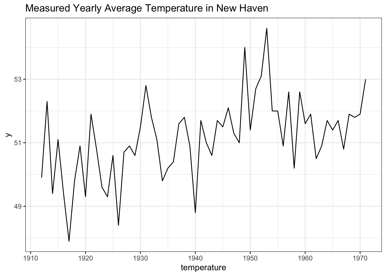

So, this dataset simply gives what the average temp for the year was from 1912 to 1971. Let’s think of this phenomenon with a Kalman Filter paradigm: the unknown state we are trying to observe is the true average yearly temperature in New Haven. This dataset provides us with our measurements of the temperature; since these measurements may be noisy, we will use the Kalman Filter to try to enhance our estimate.

We can set up our simple Kalman Filter model that we established in Equations 1 and 2:

$$\theta_t = \theta_{t - 1} + v_t$$

$$Y_t = \theta_t + w_t$$

Where, again, $v_t \sim N(0, \sigma_{v_t}^2)$ and $w_t \sim N(0, \sigma_{w_t}^2)$, where each of the $v_t$ and $w_t$ terms are independent of each other through time (and $v_t$ is independent of $w_t$). We will refer to these as the transition and measurement equations, respectively (transition because we are transitioning from $\theta_{t - 1}$ to $\theta_t$, and measurement because we are measuring the data $Y_t$).

Notice here that, for simplicity, we have $F_t = G_t = 1$ (we won’t have to worry about those constants!). Again, we can think of $\theta_t$ as the true yearly temperature in year $t$, which moves through time as we add the random noise $v_t$ at each period. We can think of $Y_t$ as the measurement of the yearly temperature that is reported in our dataset in each period (again, note that the measurement is noisy: we have the true value $\theta_t$ plus some noise $w_t$; again, the measurements are not totally accurate!).

Let’s now turn to the FKF package (specifically, the fkf function) to try to run a Kalman filter. Let’s start by matching up our variables in R.

y <- nhtemp
a0 <- y[1]
P0 <- matrix(1)

Naturally, y, our data, is coming from nhtemp. Following the fkf documentation (which you can read by typing ?fkf), we let a0 be our initial guess for $\theta$; a natural choice is just the temperature in the first period y[1]. We let P0 be our best guess for the variance of $\theta$; we use 1 here, which is close to the sample variance (var(y) gives 1.6) and is a nice round number.

We now define our next set of parameters:

dt <- ct <- matrix(0)

According to the documentation of the fkf function, these parameters give the ‘intercepts’ of the transition and measurement equations, respectively. The idea here is that we can extend our Kalman equations to add a constant that varies with time (i.e., $\theta_t = \theta_{t - 1} + d_t + v_t$, where $d_t$ is a time-varying constant) in more complicated cases. For example, if we were working with monthly average temperatures, we might want to add a time-varying constant to adjust for seasonality; however, we don’t have this sort of construction in the problem at hand (temperatures are yearly), so we simply set these variables to $0$.

Next we set our $F_t$ and $G_t$ values:

Zt <- Tt <- matrix(1)

These are labeled in the fkf documentation as the ‘factors’ of the transition and measurement equations, which are $F_t$ and $G_t$ in our parlance. We defined these to be $1$ earlier on, so we simply set them to $1$. here.

Finally, we have to set parameters HHt and GGt, which give the variance of the transition and measurement equations, or $\sigma_{v_t}^2$ and $\sigma_{w_t}^2$ in our parlance. If we peek at the documentation in the fkf function, we see that these variances are estimated by maximizing the log-likelihood of the Kalman Filter (search for fit.fkf). We can borrow this approach here:

# Estimate parameters:
fit.fkf <- optim(c(HHt = var(y, na.rm = TRUE) * .5,
                   GGt = var(y, na.rm = TRUE) * .5),
                 fn = function(par, ...)
                 -fkf(HHt = matrix(par[1]), GGt = matrix(par[2]), ...)$logLik,
                 yt = rbind(y), a0 = a0, P0 = P0, dt = dt, ct = ct,
                 Zt = Zt, Tt = Tt)


# recover values
HHt <- as.numeric(fit.fkf$par[1])
GGt <- as.numeric(fit.fkf$par[2])
HHt; GGt

## [1] 0.05051545

## [1] 1.032562

This essentially just initializes the optimizer search for HHt and GGt at half of the variance of the data y (this is the var(y, na.rm = TRUE) * .5) and searches for the values of HHt and GGt that maximizes the log likelihood (using all of the other pre-defined parameters).

Finally, then, our parameters are set, and we can run our Kalman Filter:

y_fkf <- fkf(a0, P0, dt, ct, Tt, Zt,
             HHt = matrix(HHt), GGt = matrix(GGt),
             yt = rbind(y))

From the documentation of fkf, we have that y_fkf$att is the filtered state variables (our guess for $\theta_t$, the true temperature, given the data $Y_t$ that we observe) and y_fkf$at is the predicted state variables (our guess for $\theta_{t + 1}$ given the data $Y_t$ that we observe). We are interested here in the filtered variable, so we can plot it:

data <- data.table(x = seq(from = 1912, to = 1971, by = 1),
                   y = as.numeric(nhtemp),
                   y_kalman = as.numeric(y_fkf$att))


ggplot(data, aes(x = x, y = y)) +
  geom_line() +
  geom_line(data = data, aes(x = x, y = y_kalman), col = "blue") +
  xlab("year") + xlab("temperature") +
  ggtitle("Measured Yearly Average Temperature in New Haven (with Kalman Filter)") +
  theme_bw()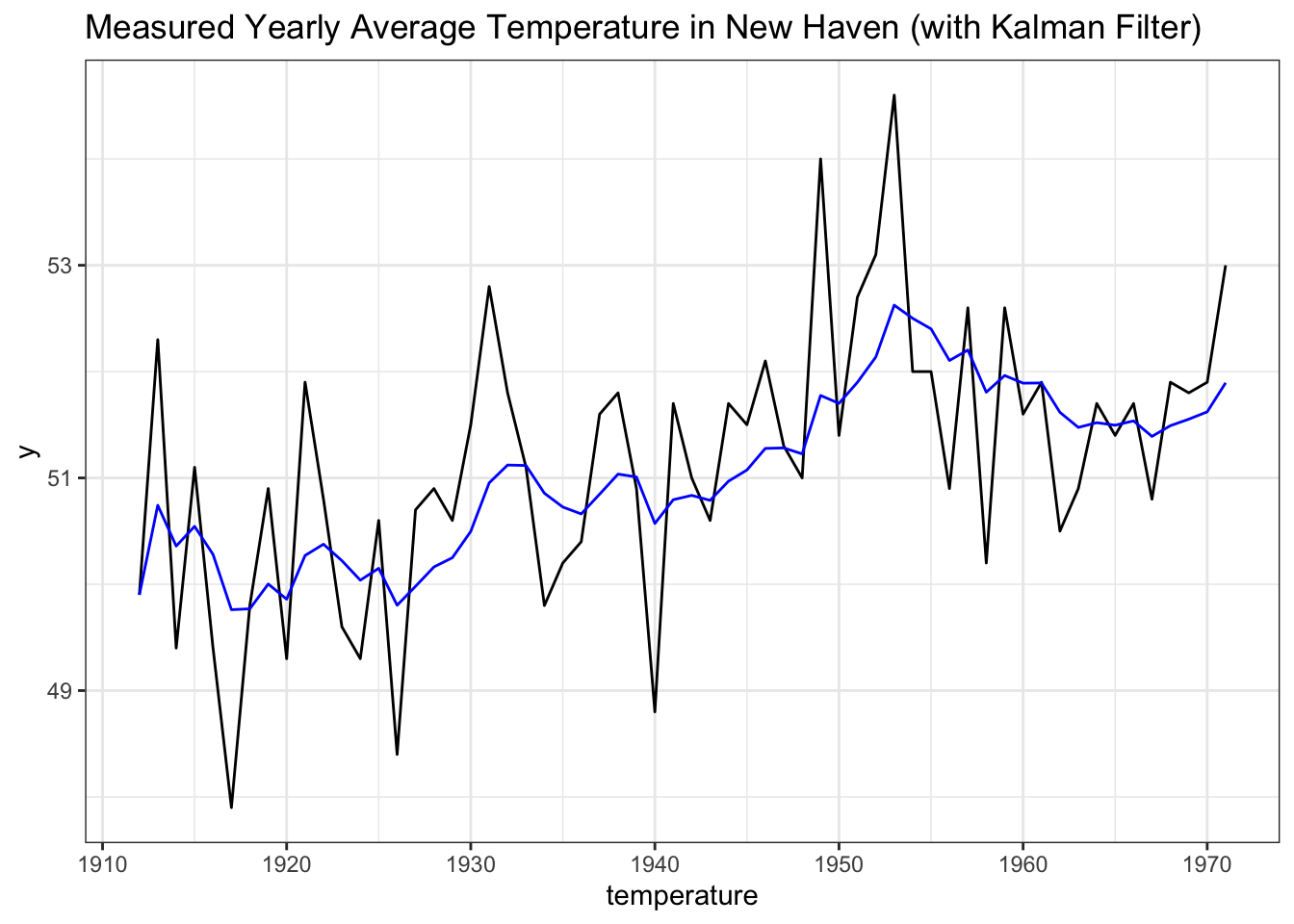

Excellent! The blue line is the estimate for what the true temperature, while the black lines are the (potentially noisy) measurements that we observe.

It is great that we can use the fkf package to run a Kalman Filter, but we should try brute forcing a solution from the ground up using our algebraic derivation. Recall our final result:

$$\theta_t | Y_1, ..., Y_{t - 1}, e_t \sim N(G_t\hat{\theta}_{t-1} + R_t F_t^{\prime}(\sigma_{v_1} ^ 2 + F_t R_t F^{\prime}_t)^{-1}e_t,$$ $$R_t - R_tF^{\prime}_t(\sigma_{v_t}^2 + F_tR_tF^{-1}_t)^{-1}F_tR_t)$$

Where $R_t = G_t\Sigma_{t - 1} G^{\prime}_t + \sigma_{w_t}^2$.

We can try to use this ground-up derivation to reproduce the output from the fkf function. Let’s set up paths for the state variable (theta) and its variance (theta_var), loop through and calculate the estimates. Note that we can employ the parameters a0, p0, Zt, Tt, HHt, and GGt that we used in the fkf output (we will even convert them to the notation of Equation 11 so it’s easier to match with our algebraic solution).

# initialize
theta <- theta_var <- rep(NA, length(y) + 1)

# set our initial guess
theta[1] <- a0
theta_var[1] <- P0

# define parameters (notation consistent with Equation 11).
sigma_w <- sqrt(HHt)
sigma_v <- sqrt(GGt)
G_t <- Tt
F_t <- Zt

# iterate and make estimates
for (i in 1:length(y)) {
  
  # Equation 6.
  # use previous theta value for theta_hat and calculate e_t
  theta_hat <- theta[i]
  e_t <- y[i] - theta_hat * G_t * F_t
  
  # calculate R_t
  R_t <- G_t * theta_var[i] * G_t + sigma_w ^ 2
  
  # generate estimates from Equation 11
  theta[i + 1] <- G_t * theta_hat + R_t * F_t * (sigma_v ^ 2 + F_t ^ 2 * R_t) ^ (-1) * e_t
  theta_var[i + 1] <- R_t - R_t * F_t * (sigma_v ^ 2 + F_t ^ 2 * R_t) ^ (-1) * F_t * R_t
}

# adjust by one
theta <- theta[-1]
theta_var <- theta_var[-1]

We thus were able to run the Kalman Filter from the ground up, using our algebraic result. Does it match what we got from the fkf package?

data <- data.table(x = seq(from = 1912, to = 1971, by = 1),
                   y = as.numeric(nhtemp),
                   y_kalman = as.numeric(y_fkf$att),
                   y_algebra = theta)


ggplot(data, aes(x = x, y = y)) +
  geom_line() +
  geom_line(data = data, aes(x = x, y = y_kalman), col = "blue", alpha = 1 / 2) +
  geom_line(data = data, aes(x = x, y = y_kalman), col = "red", alpha = 1 / 2) +
  xlab("year") + xlab("temperature") +
  ggtitle("Measured Yearly Average Temperature in New Haven (with Kalman Filter)") +
  theme_bw()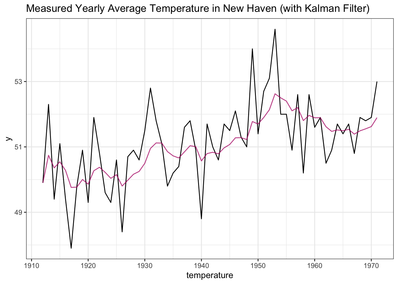

Excellent! Our output is the exact same as the fkf output (the red and blue lines are overlaid with alpha = 1/2, which is why we just see a purple line). This validates all of that intense algebra that we did; it’s easy to code up the result and show that it matches what’s going on behind the scenes in the fkfpackage!