Chapter 7 Black Scholes
“Time is money.” -Benjamin Franklin

Motivation
This chapter will explore another practical application of Stochastic Processes, specifically in a financial context. Even readers that don’t have interest in quantitative finance may find the derivation and result of Black Scholes interesting.
7.1 Black Scholes Model
The Black Scholes Model, most often just referred to as ‘Black Scholes,’ is one of the most widely used mathematical applications of stochastic processes (and, of course, other fields in Statistics!). It was derived by Fischer Black and Myron Scholes to model a key phenomenon in the financial world.
We’re going to need a little bit of background on some financial concepts before diving in to Black Scholes. You’re probably familiar with what a ‘stock’ is: basically a share of ownership in a company that you can buy and sell on some market (naturally, these shares of ownership usually do better when the company is doing well!). Apple stock, which is traded with the ‘ticker’ (essentially an ID for the stock) of ‘AAPL,’ is a common example. We can easily get historical values for the stock price of AAPL with the quantmod package:
library(quantmod)

# saves an object called AAPL
getSymbols("AAPL")
## [1] "AAPL"# view results
head(AAPL)## AAPL.Open AAPL.High AAPL.Low AAPL.Close AAPL.Volume AAPL.Adjusted
## 2007-01-03 3.081786 3.092143 2.925000 2.992857 1238319600 2.573566
## 2007-01-04 3.001786 3.069643 2.993571 3.059286 847260400 2.630688
## 2007-01-05 3.063214 3.078571 3.014286 3.037500 834741600 2.611954
## 2007-01-08 3.070000 3.090357 3.045714 3.052500 797106800 2.624853
## 2007-01-09 3.087500 3.320714 3.041071 3.306071 3349298400 2.842900
## 2007-01-10 3.383929 3.492857 3.337500 3.464286 2952880000 2.978950We won’t get into what all of these columns mean; for now, we can focus on AAPL.Close, which is simply how much one share of Apple cost when the market closed each day. Let’s visualize the price over time:
data <- data.table(date = index(AAPL),
                   price = as.numeric(AAPL$AAPL.Close))

ggplot(data, aes(x = date, y = price)) +
  geom_line() +
  xlab("") + ylab("price") + ggtitle("Apple Stock Price") +
  theme_bw()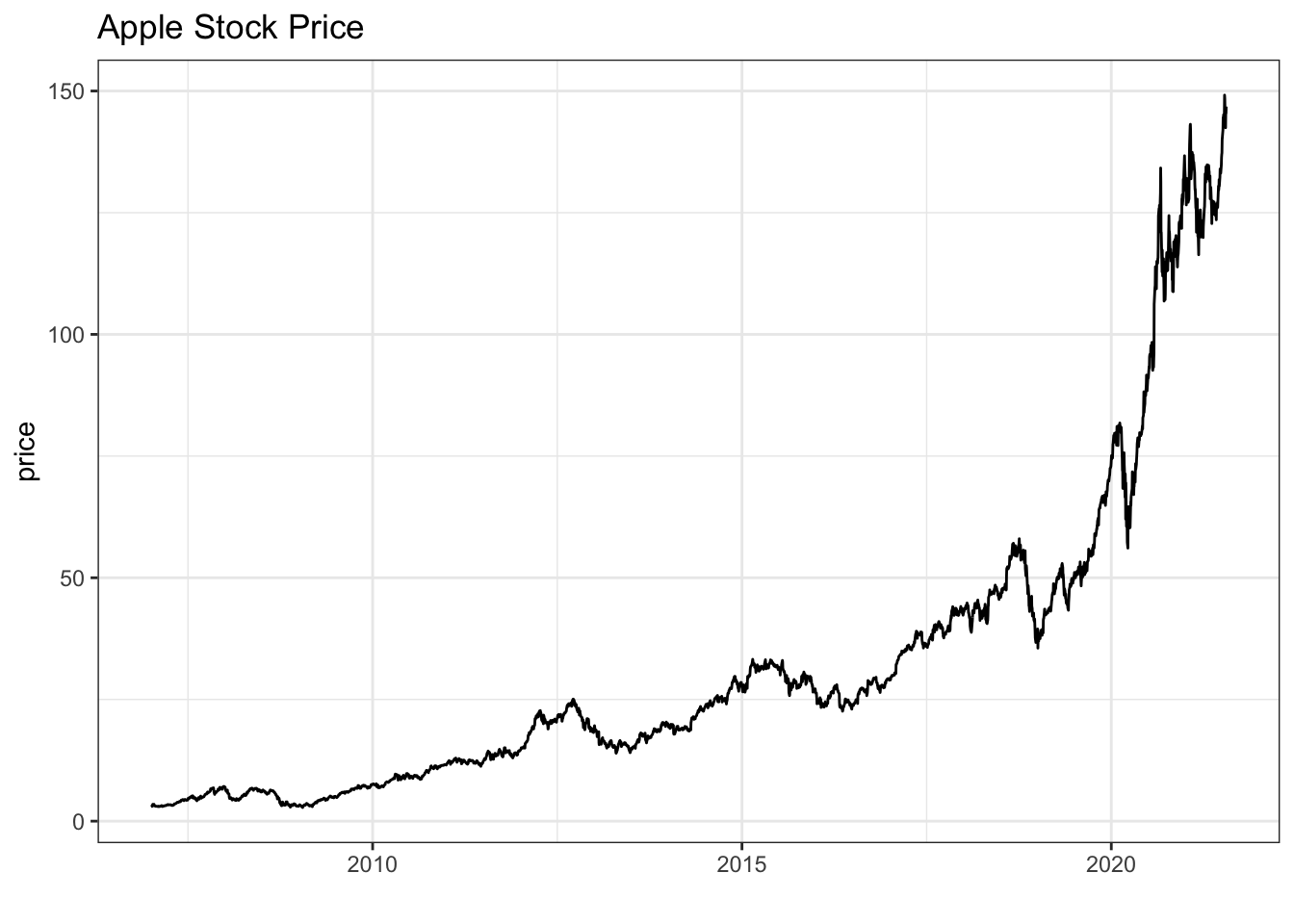
We’re, familiar, then, with the concept of stocks; we’re going to introduce the concept of Call Options. Here’s a video introduction:
Click here to watch this video in your browser
Don’t worry; if videos aren’t your thing, we’ll work through call options in long form. Let’s start with an example of a simple stock (that we simulate; simply for illustration purposes, we will start at \(\$20\) and simulate from a Normal distribution with a mean of \(.1\)):
# replicate
set.seed(0)

# generate data
S <- round(cumsum(c(20, rnorm(99, mean = .1))), 2)

# visualize
data <- data.table(t = 1:length(S),
                   S = S)

ggplot(data, aes(x = t, y = S)) +
    geom_line() +
    theme_bw() +
    xlab("") + ylab("Price") +
    ggtitle("Stock Price over time")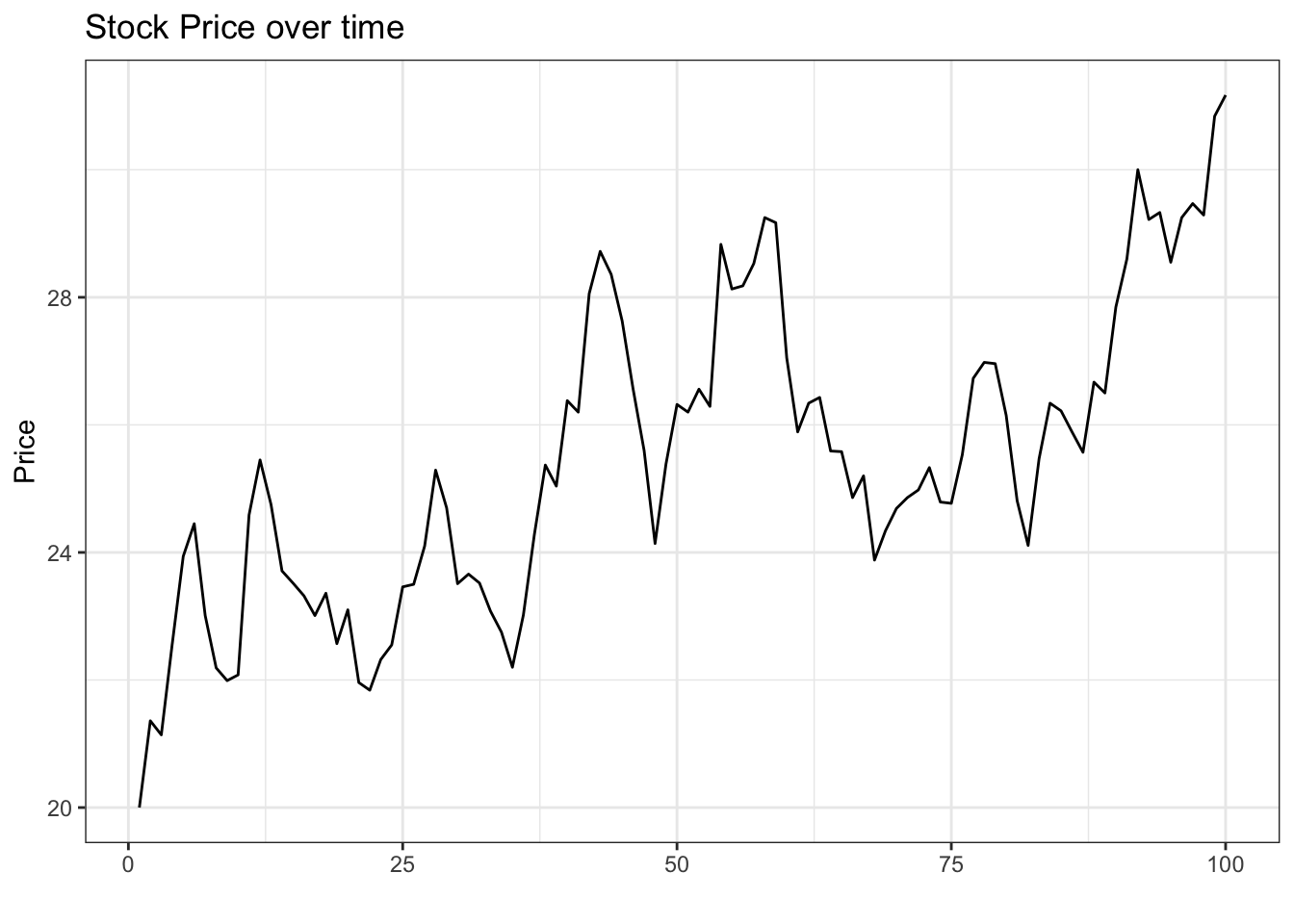
Not too bad; after \(100\) days, the stock price has risen to \(\$31.17\). Now let’s define a simple call option, which is a contract that gives you the option to purchase a stock for a specified amount on a specified date. One example would look like this:
Contract A: Call option struck at \(\$35\) expiring on day 125
This simply means that, if you own the call option, you have the option to buy the stock for \(\$35\) (this is called the strike price or just the strike) on day 125 (this is called the maturity or expiry; some options allow you to buy the stock at different points in time, including any time up to the maturity, but we will only be dealing with options that allow you to buy the stock at the maturity).
This sounds kind of strange; why on Earth would we want the option to buy something? Well, let’s say that you expect the stock to be worth \(\$40\) on day 125. You could then, as stated in the contract, ‘exercise’ your option and buy the stock for \(\$35\) (note that this is below the current market price of \(\$40\), you only get the right to buy it at a lower price because you own the option) and turn around and sell it to for the current market price of \(\$40\) for a quick \(\$5\) profit (you could also hold onto the stock, of course, after you bought it). If things didn’t work out and the stock price fell to \(\$27\) on day 125, then you just simply wouldn’t exercise your option and it would ‘expire’ (you wouldn’t buy the stock for the \(\$35\) stated on the option contract, since you could just buy it for \(\$27\), or the normal market price).
Therefore, intuitively, the call option gives you the option to buy the stock in the case that the stock price goes higher than strike (and thus make a profit). If the stock ends up above the strike price - and thus we exercise our option - we say that the option is in the money. Naturally, if the stock ends below the strike place, we say it is out of the money and we don’t exercise our option (if the stock ends exactly at the strike price, we say that it is at the money).
The key question is: how much would you pay for Contract A?
At first, you’re probably juggling a bunch of initial questions: what is the probability that the stock ends up ‘in the money’ (above the strike price so that we can exercise the option), so that the option isn’t worthless? If the stock does end up in the money, how much will it be in the money?
For starters, to get some intuition on valuing options, let’s compare Contract A to a couple of other call options (all derived on the same stock from above; call options are called derivatives for exactly this reason, as their value is derived from some underlying financial asset - here, the stock).
Contract A: Call option struck at \(\$35\) expiring on day 125
Contract B: Call option struck at \(\$40\) expiring on day 125
Contract C: Call option struck at \(\$35\) expiring on day 110
Let’s think about the relative prices of these contracts. First, which contract is more valuable (should be more expensive): Contract A or B?
The two contracts are identical except for their strike; Contract A has a strike of \(\$35\) and Contract B has a strike of \(\$40\). Which option would you pay more for?
Since because, simply put, \(\$40\) is more than \(\$35\), the stock has to go higher for Contract B to be ‘in the money’; it is thus harder for us to exercise Contract B and profit off of it. Further, remember, that if we are exercising Contract B (i.e., the stock price is above \(\$40\)), we could also be exercising Contract A and would make \(\$5\) more! Therefore, Contract A should be more expensive than Contract B (we will see how much more expensive soon).
How about Contract A and Contract C? The only difference here is the expiry; Contract C expires sooner than Contract A (they have the same strike). Which one would you pay more for?
This one is a bit more tricky. The relevant question is straightforward: is it good to have a longer expiry in an option?
This isn’t immediately obvious. In this example, the stock is at around \(\$30\) at time \(t = 100\). For Contract C, the stock would have to get to the strike of \(\$35\) (and thus be in the money) by time \(t = 110\); for Contract B, the stock has until \(t = 125\) to get there. However, although it has more time to move upwards in price (and therefore be in the money), it also has more time to move downwards. One could envision a path where the stock price was worth \(\$38\) at time \(t = 110\), thus making Contract B in the money, and then falls to \(\$32\) by time \(t = 125\), making Contract A out of the money. Ultimately, more time could be good or bad.
The answer - which we will see over and over in this chapter - lies in the fact that there is unlimited upside compared to limited downside. In the absolute worst case scenario, the call option is worth zero (the stock is below the strike at expiry). However, theoretically, the stock price could go up infinitely, and thus the price of the call option could also go up infinitely (if you aren’t satisfied with the intuition of infinity, substitute in that the stock could instead just go very, very high and thus the option value could go very, very high). Because we have enormous, essentially unlimited upside and capped downside, more time is good. We want to let our stock bounce around for as long as possible, because, while our losses have a limit, there is a chance that we could win really big.
Now that we have a handle on some of the major factors that make call options more or less valuable, let’s turn to the major topic of this chapter.
7.2 Deriving Black Scholes
The Black Scholes Model is, simply put, a way to value (i.e., put a price on) the options that we discussed above. By using a few assumptions, the model can easily spit out prices for options given a few input parameters (some of which we have already seen, including the current stock price, time until expiry and strike price). Black Scholes is a relevant study here because it makes liberal use of stochastic processes and other statistical tools in general. We can work through the derivation now, adapted from Stephen Blyth’s Introduction to Quantitative Finance.
7.2.1 Log-Normal
We can start the derivation by learning about a new distribution: the Log-Normal distribution. This distribution is so named because, for example, if \(Y\) is Log-Normal, then the log (natural log, that is) of \(Y\) is Normal. That is, if \(Y\) is Log-Normal with parameters \(\mu, \sigma^2\), then \(ln(Y) \sim N(\mu, \sigma^2)\), or \(X \sim N(\mu, \sigma^2)\) where \(Y = e^X\) (or \(ln(Y) = X\)).
Let’s try to get comfortable with the distribution by calculating the mean and variance. For the mean, we will start with a standard Normal \(Z \sim N(0, 1)\). By the definition above, \(e^{Z}\) is Log-Normal (the log of \(e^Z\) is \(Z\), which is Normal). Let’s use LOTUS to calculate the expectation of \(e^Z\) (just the function \(e^z\) multiplied by the PDF of a standard Normal \(f(x)\) and integrated over the entire support):
\[E(e^Z) = \int_{-\infty}^{\infty} e^z f(z)dz\] \[= \frac{1}{2 \pi} \int_{-\infty}^{\infty} e^z e^{\frac{-z^2}{2}}dz\] \[\frac{1}{2 \pi} \int_{-\infty}^{\infty} e^{z + \frac{-z^2}{2}}dz\]
We thus have \(z - \frac{z^2}{2}\) in the exponent. We can try completing the square by adding and subtracting \(\frac{1}{2}\):
\[z - \frac{z^2}{2}=z - \frac{z^2}{2} + \frac{1}{2} - \frac{1}{2}\]
We can multiply and divide \(z\) by \(2\) to get a common denominator:
\[=(\frac{2z}{2} - \frac{z^2}{2} - \frac{1}{2}) + \frac{1}{2}\]
\[=(\frac{-z^2 + 2z - 1}{2}) + \frac{1}{2}\]
Adjusting signs:
\[=-(\frac{z^2 - 2z + 1}{2}) + \frac{1}{2}\]
And finally completing the square:
\[=-\frac{(z - 1)^2}{2} + \frac{1}{2}\]
We can go ahead and plug this back into our numerator in the LOTUS calculation:
\[\frac{1}{2 \pi} \int_{-\infty}^{\infty} e^{-\frac{(z - 1)^2}{2} + \frac{1}{2}}dz\] Factoring out the \(e^{\frac{1}{2}}\):
\[=e^{\frac{1}{2}} \Big(\frac{1}{2 \pi} \int_{-\infty}^{\infty} e^{-\frac{(z - 1)^2}{2}}dz\Big)\] Note that the integral (with the constant \(\frac{1}{2\pi}\)) is now just the PDF of a \(N(1, 1)\) random variable, integrated over the support! That is, it simply goes to 1. We are thus just left with:
\[E(e^Z) = e^{\frac{1}{2}}\]
Excellent; we have found the mean of \(e^Z\). Now let’s turn towards finding the mean of \(e^X\), where \(X \sim N(\mu, \sigma^2)\). We can start by remembering that \(X \sim \sigma Z + \mu\) (for a quick check, remember that a linear combination of Normals is Normal, so \(\sigma Z + \mu\) is Normal, and then calculate the mean and variance of \(\sigma Z + \mu\) to show that you get \(\mu\) and \(\sigma^2\)) and plugging this in:
\[E(e^X) = E(e^{\mu + \sigma Z}) = e^{\mu} E(e^{\sigma Z})\]
Let’s use a similar approach to calculate \(E(e^{\sigma Z})\); LOTUS gives us:
\[E(e^{\sigma Z}) = \frac{1}{2 \pi} \int_{-\infty}^{\infty} e^{\sigma z} e^{\frac{-z^2}{2}}dz\]
Again, we can look at the exponent and complete the square:
\[\sigma z - \frac{-z^2}{2}\]
\[ = (\sigma z - \frac{-z^2}{2} - \frac{\sigma^2}{2}) + \frac{\sigma^2}{2}\]
\[ = (\frac{2\sigma z}{2} - \frac{-z^2}{2} - \frac{\sigma^2}{2}) + \frac{\sigma^2}{2}\]
\[= -(\frac{z^2 - 2\sigma z + \sigma^2}{2}) + \frac{\sigma^2}{2}\]
\[=-(\frac{z - \sigma}{2}) + \frac{\sigma^2}{2}\] Plugging back in:
\[E(e^{\sigma Z}) = \frac{1}{2 \pi} \int_{-\infty}^{\infty} e^{-(\frac{z - \sigma}{2}) + \frac{\sigma^2}{2}}dz\] \[=e^{\frac{\sigma^2}{2}} \Big(\frac{1}{2 \pi} \int_{-\infty}^{\infty} e^{-(\frac{z - \sigma}{2})}dz\Big)\] Again, we can use the fact that the integral (with the \(\frac{1}{2 \pi}\)) is just the integral of the PDF of a \(N(\sigma, 1)\) random variable, which integrates to \(1\). We are left with:
\[E(e^X) = e^{\mu} E(e^{\sigma Z}) = e^{\mu + \frac{\sigma^2}{2}}\]
Voila! We have calculated the mean of \(e^X\), which is Log-Normal. Here’s a video walkthrough of this process:
Click here to watch this video in your browser
Let’s now turn to the variance; we have actually already done most of the leg work. Again, let \(X \sim N(\mu, \sigma^2)\) so that \(Y = e^X\) is Log-Normal by definition. We can look to calculate the variance:
\[Var(e^X) = E\big((e^X)^2\big) - E(e^X)^2\]
We know that \(E(e^X) = e^{\mu + \frac{\sigma^2}{2}}\) from the first part, and we know that \(E((e^X)^2) = E(e^{2X})\). Note that \(2X \sim N(2\mu, 4 \sigma^2)\) (again, a linear combination of a Normal is Normal, so a linear combination of \(X\) is Normal; it should be straightforward to show that \(2X\) has a mean of \(2 \mu\) and a variance of \(4 \sigma^2\)), so we can just use our formula for the mean of a Log-Normal (just plugging in \(2\mu\) for the mean and \(4\sigma^2\) for the variance):
\[Var(e^X) = e^{2\mu + \frac{4 \sigma^2}{2}} - (e^{\mu + \frac{\sigma^2}{2}})^2\]
\[= e^{2\mu + 2 \sigma^2} - e^{2 \mu + \sigma^2}\]
Factoring out:
\[Var(e^X)=e^{2\mu + \sigma^2}\big(e^{\sigma^2} - 1\big)\]
Excellent! To recap, we have shown that, if \(Y\) is Log-Normal with parameters \(\mu, \sigma^2\), we have:
\[E(Y) = e^{\mu + \frac{\sigma^2}{2}}\] \[Var(Y)=e^{2\mu + \sigma^2}\big(e^{\sigma^2} - 1\big)\]
For a video explanation, see below:
Click here to watch this video in your browser
The Log-Normal is useful in finance because the support is non-negative (this makes sense, because the Log-Normal is just the log of something, and the log of something is non-negative). Therefore, for modeling stocks, which cannot have a negative price, the Log-Normal can be more useful than the Normal (who’s support is the entire real line).
We can easily simulate the Log-Normal in R like we would with other distributions (rlnorm is the function that generates random values). Note that the mean and standard deviation parameters we input are equivalent to our set-up above; that is, if we input 2 as the mean in rlnorm, we are saying that this is a random variable that, if logged, is Normal with mean 2. Let’s generate some examples to explore this relation (and test our results for the mean and variance!).
# replicate
set.seed(0)


# initialize parameters
n <- 1000
mu <- 3
sigma <- .7

# generate data
X <- rnorm(n, mu, sigma)
X_log <- rlnorm(n, mu, sigma)

# visualize
ggplot() +
  geom_histogram(aes(X_log)) +
  theme_bw() + ggtitle("Log-Normal")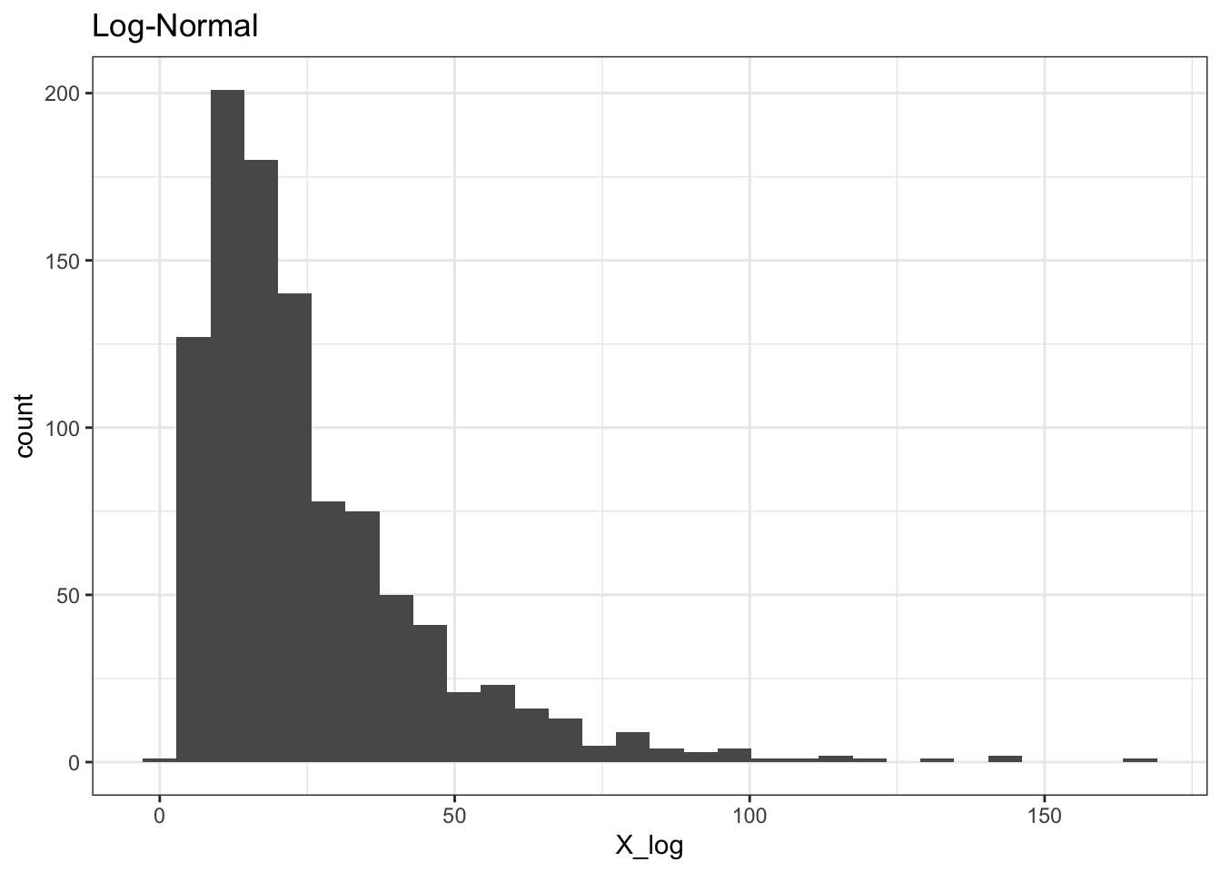
# visualize log of Log-Normal
ggplot() +
  geom_histogram(aes(log(X_log)), fill = "red", alpha = 1 / 2) +
  geom_histogram(aes(X), fill = "blue", alpha = 1 / 2) +
  theme_bw() + ggtitle("Log of Log-Normal and Normal") +
  xlab("value")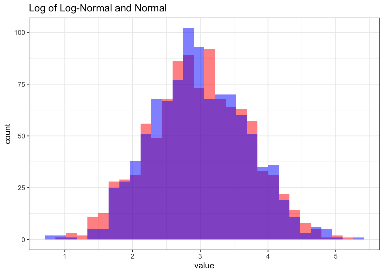
# check results
mean(X_log); exp(mu + sigma ^ 2 / 2)
## [1] 25.56843## [1] 25.66171var(X_log); exp(2 * mu + sigma ^ 2) * (exp(sigma ^ 2) - 1)## [1] 408.2131## [1] 416.395Excellent! It looks like, as we discussed, the Log-Normal has a non-negative support (first chart), the log of the Log-Normal seems to match the Normal with the same parameters (second chart with two histograms) and the results that we found for the mean and variance are close to what we observed empirically!
7.2.2 Risk-Neutral Paradigm
Let’s now get back to the financial part of this derivation. We will define the price of a stock at time \(t\) as \(S_t\) (note that this is a stochastic process!). Imagine that, in a single period (i.e., from \(t\) to \(t + 1\)), the stock either goes to \(S_t(1 + u)\) or \(S_t(1 + d)\). The letter \(u\) simply stands for ‘up’ and \(d\) simply stands for ‘down,’ so we have:
\[u > d\] \[S_t(1 + u) > S_t(1 + d)\]
Note that \(u\) doesn’t necessarily have to be positive (or \(d\) be negative), it just has to be greater than \(d\).
Anyways, one potential example would be \(u = .01\) and \(d = -.01\). Therefore, for each step, the stock either goes up 1% (we have \(S_t(1 + .01)\)) or down by 1% (we have \(S_t(1 - .01)\))
Now we can introduce the concept of the risk free rate, which we will denote as \(r\). This is the rate that we can lend at for each period.
If this is confusing, let’s think of a simple example where \(r = .02\). This means that the risk free rate is 2%. If you lent \(\$100\) at time \(t = 1\) at the risk free rate, then you would get back \((1 + .02)100 = 102\) dollars at time \(t = 2\) (over one period). Over \(n\) periods, you would get back \((1 + .02)^n \cdot 100\) dollars.
In our current example with \(u\) and \(d\) as the up and down moves of our stock, we must have:
\[d < r < u\]
To show this, we are going to have to introduce the No-Arbitrage Principle. As this is not a book on quantitative finance, we won’t delve too deeply into the mathematics behind this principle, just the definition.
For our purposes, we can define arbitrage as riskless profit above the risk free rate. Let’s see a simple example. Imagine that the risk free rate is \(r = .02\), so that in one period you earn, without any risk, 2%. Now imagine a stock with \(u = .04\) and \(d = .03\); that is, the stock either goes up 3% or up 4%. If this were the case, one could borrow 100 dollars at the risk free rate of \(.02\) and invest that 100 dollars in the stock. After one period, we owe \(\$102\) (we borrowed \(\$100\) at the risk free rate of \(.02\)) but, thankfully, the stock has either gone up to \(\$103\) or \(\$104\), so we can sell the stock, pay back our loan and still profit \(\$1\) or \(\$2\).
Therefore, this investment strategy locked in a guaranteed profit of one or two dollars (this strategy is riskless because there is no chance of losing money). Still, it’s not clear that the investor makes more than the risk free rate here; isn’t he just making \(\$1\) or \(\$2\), which is still less than or equal to the \(\$2\) he would make from the risk free rate?
This is where the idea of leverage comes in, or borrowing extra money to amplify the outcomes of the investment strategy. Remember, in the above example, the investor isn’t putting up his own money; he is borrowing the 100 dollars and then investing that 100 dollars in the stock. Therefore, for \(0\) dollars put up, the investor is making a guaranteed return . What’s more, the investor could borrow and thus invest \(\$100,000\) in this strategy, driving returns up to \(\$100\) or \(\$200\), still for \(\$0\) actually put up. Theoretically, there’s no real upper limit to what the investor could borrow and invest in this strategy, and, if all of his returns are based of zero dollars invested, then his ‘rate of return’ is way better than the risk free rate (instead of just making \((1 + r)\) on the money he invested, he is making tons of money on zero dollars actually invested).
If this is confusing, check out this video on arbitrage:
Click here to watch this video in your browser
In real life, in situations like this, the extra demand for the stock would drive the stock price up and thus correct any arbitrage (savvy investors would ‘arbitrage-out’ any mispricings). For our purposes, we will be satisfied with the result that no arbitrage is allowed in the construction of our scenarios.
Above we saw the case where \(r < d < u\). What about the case where \(d < u < r\), or the risk free rate is higher than both \(u\) and \(d\)? It’s harder to see what an investor would do in this case, but it essentially the opposite of the previous example. Instead of buying or ‘going long’ the stock, the investor shorts the stock (borrows the stock, sells it for cash and promises to buy it back the next period). Let’s say the stock is worth \(\$100\); the investor borrows the stock, sells it for \(\$100\) cash and invests that cash in the risk free rate. In the next period, the investor has \(100(1 + r)\) (the \(\$100\) cash times what that cash earned from the risk free rate), and buys back the stock (remember, he borrowed it!), either at \(100(1 + u)\) dollars or \(100(1 + d)\) dollars. Since \(d < u < r\), we have that \(100(1 + d) < 100(1 + u) < 100(1 + r)\), and thus the investor makes some positive profit. Again, the investor put no cash of his own down up front and, again, the investor could potentially lever up this investment massively; therefore, the investor is doing much better than the risk free rate with this arbitrage strategy.
Therefore, we must have that \(d < r < u\), which of course means \((1 + d) < (1 + r) < (1 + u)\). The first of our two arbitraging investors above would lose money in a down move, since he would have to pay back the \(1 + r\) loan, which is more money than the \(1 + d\) price of the stock he owns. The second investor would lose money in an up move, since he would have to buy back the \(1 + u\) priced stock, which is more than the \(1 + r\) he got from investing in the risk free rate. That is, both strategies now have risk of losing money; they are no longer just making riskless profit.
Let’s finally turn to what the risk-neutral probability means in this context. Simply put, if we define \(p_*\) as the risk neutral probability, then \(p_*\) is the probability of the stock taking the ‘up move’ and \(1 - p_*\) is the probability of the stock taking the ‘down move’ such that the expectation of the value of the stock at time \(t + 1\) equals \(S_t(1 + r)\). More formally:
\[E(S_{t+1}|S_t) = p_*S_t(1 + u) + (1 - p_*)S_t(1 + d) = (1 + r)S_t\]
We can then solve for \(p_*\). Dividing by \(S_t\), we have:
\[ p_*(1 + u) + (1 - p_*)(1 + d) = (1 + r)\]
\[=p_*(1 + u) - p_*(1 + d) + (1 + d) = (1 + r)\]
\[=p_* + up_* - p_* - dp_* + 1 + d = 1 + r\]
\[=p_*(u - d) + d + 1 = 1 + r\]
\[=p_*(u - d) + d = r\] \[=p_*= \frac{r-d}{u - d}\]
So, if the probability of an ‘up move’ is \(\frac{r-d}{u - d}\) (and the probability of a ‘down move’ is \(1 - \frac{r-d}{u - d}\)), then the expectation of the price stock in the next period is equal to how much cash you would make if you just lent the dollar price of the stock \(S_t\) at the risk free rate for one period.
The risk-netural paradigm can be tricky; here is a video to solidify the concept.
Click here to watch this video in your browser
7.2.3 Symmetric Stock
We’ve constructed our stock \(S_t\) that either has an ‘up move’ to \((1 + u)S_t\) or a ‘down move’ to \((1 + d)S_t\) after one period. In this section, let’s imagine that the stock has an up move with probability \(1/2\) and a down move with probability \(1/2\) (we learned about the risk neutral probability in the previous section; this \(1/2\) is not necessarily the risk neutral probability, and we will return to the more general risk neutral probability soon).
Let’s define the ‘log return’ at time \(t + 1\) as simply:
\[\lambda_{t + 1} = log(\frac{S_{t + 1}}{S_t})\]
Or, simply put, the log of the stock price in period \(t + 1\) divided by the stock price in period \(t\).
Let’s imagine that we are at time \(t\), and thus \(S_t\) is known; from above, we have that \(S_{t + 1}\) is a random variable that takes on the value \((1 + u)S_t\) with probability \(1/2\) and takes on the value \((1 + d)S_t\) with probability \(1/2\).
This means that \(\lambda_{t + 1}\) is a random variable as well. In the case of an up move, we have that:
\[\lambda_{t + 1} = log(\frac{S_t(1 + u)}{S_t}) = log(1 + u)\]
And, similarly, in the case of a down move, we have:
\[\lambda_{t + 1} = log(\frac{S_t(1 + d)}{S_t}) = log(1 + d)\]
Therefore, \(\lambda_{t + 1}\) is just a random variable that takes on the value \(1 + u\) with probability \(1/2\) and the value \(1 + d\) with probability \(1/2\).
Let’s now think about the stock across many periods. Let each period have length \(\Delta T\) (so that the difference between periods in time is \(\Delta T\) and that there be \(N\) total periods). Define \(T\) as the total amount of time that passes, so that we have \(T = N \cdot \Delta T\) (the total amount of time that passes is the length of one interval times the total number of intervals).
Now let’s define \(Y_T\) as the ‘log return’ of the stock up to period \(T\). We have:
\[Y_T = log(\frac{S_T}{S_0})\]
Where \(S_T\) is the price of the stock at time \(T\) and \(S_0\) is the initial price of the stock. Since \(Y_T\) is a function of the random variable \(S_T\) (we take \(S_0\) as given), we know that \(Y_T\) is a random variable; for now, let us say that \(E(Y_T) = \mu T\) and \(Var(Y_T) = \sigma^2 T\) for some \(\mu\) and \(\sigma^2\) (we will come back to this later, but let us take these definitions as given for now).
Because of the properties of the log, we can expand out \(Y_T\) as a summation:
\[Y_T = log(\frac{S_{(\Delta T)}}{S_0}) + log(\frac{S_{(2\Delta T)}}{S_{(\Delta T)}}) + ... + log(\frac{S_{N (\Delta T)}}{S_{(N - 1)(\Delta T)}})\] Because, remember, the periods of this process are at times \(0, \Delta T, 2 \Delta T, ..., N \Delta T\).
Note that the values in this summation are just the log returns, or \(\lambda\) values, that we defined earlier, so we can plug these in:
\[Y_T = \lambda_1 + \lambda_2 + ... + \lambda_N\]
Because, remember, we have \(N\) total periods (each with a length of \(\Delta T\)).
Recall that we defined the mean of \(Y\) as \(\mu T\) and the variance as \(\sigma^2 T\). We can use this (and the fact that, by symmetry, the \(\lambda\) random variables must have the same distribution; the process by which the stock moves is the same in each period) to find the expectation of each \(\lambda\) value.
\[E(Y_T) = \mu T = E(\lambda_1 + \lambda_2 + ... + \lambda_N)\]
\[\mu T= NE(\lambda_1)\]
\[E(\lambda_1) = \frac{\mu T}{N}\]
And, because each \(\lambda\) term has the same distribution (and using the fact that \(\frac{T}{N} = \Delta T\)), we have:
\[E(\lambda_i) = \mu \Delta T\]
For \(i = 1, 2, ..., N\).
Similarly, we can find the variance:
\[Var(Y_T) = T \sigma^2 = Var(\lambda_1 + \lambda_2 + ... + \lambda_N)\] \[= T\sigma^2 = NVar(\lambda_1)\]
\[Var(\lambda_i) = \sigma^2 \Delta T\]
For \(i = 1, 2, ..., N\).
We now have the mean and variance of each \(\lambda\) term. Further, we still know that each \(\lambda\) is a random variable that only takes on two values, each with probability \(1/2\). Above, we said that these values are \(log(1 + u)\) and \(log(1 + d)\). However, using the expectation and variance of each \(\lambda\) term, we can solve for what these values are in terms of \(\mu\), \(\Delta T\) and \(\sigma^2\). Specifically, we have that:
\[\lambda_i = \mu \Delta T + \sigma\sqrt{\Delta T}\]
In an up move, and…
\[\lambda_i = \mu \Delta T - \sigma\sqrt{\Delta T}\]
In a down move.
We can quickly test that these values are legitimate: a random variable that takes on \(\mu \Delta T + \sigma\sqrt{\Delta T}\) with probability \(1/2\) and \(\mu \Delta T - \sigma\sqrt{\Delta T}\) with probability \(1/2\) will clearly have a mean of \(\mu \Delta T\) (multiply each value by \(1/2\) and sum them; the \(\sigma\sqrt{\Delta T}\) term cancels out and we are left with \(\mu \Delta T\)) and a variance of \(\sigma^2 \Delta T\) (the average distance from the mean \(\mu \Delta T\) for the two values is just \(\sigma\sqrt{\Delta T}\), and we square this to get back to the variance). Therefore, we have:
\[log(1 + u) = \mu \Delta T + \sigma\sqrt{\Delta T}\] \[log(1 + d) = \mu \Delta T - \sigma\sqrt{\Delta T}\]
Let’s use this result to expand our formula for, say, \(S_{N\Delta T}\). Remember that in an up move we have:
\[S_{N\Delta T} = (1 + u)S_{(N - 1)\Delta T}\]
Taking the log, we get:
\[log(S_{N\Delta T}) = log(S_{(N - 1)\Delta T}) + log(1 + u)\]
Plugging in \(\mu \Delta T + \sigma\sqrt{\Delta T}\) for \(1 + u\), we get:
\[log(S_{N\Delta T}) = log(S_{(N - 1)\Delta T}) + \mu \Delta T + \sigma\sqrt{\Delta T}\]
In an up move. We will now use some lazy notation:
\[log(S_{N\Delta T}) = log(S_{(N - 1)\Delta T}) + \mu \Delta T \pm_* \sigma\sqrt{\Delta T}\]
Where our lazy notation, \(\pm_*\), simply means ‘plus \(\sigma\sqrt{\Delta T}\) with probability \(1/2\) or minus \(\sigma\sqrt{\Delta T}\) with probability \(1/2\)’ (i.e., an up or down move, each with probability \(1/2\)). We know have a recursive equation and could plug in for \(log(S_{(N - 1)\Delta T})\) in terms of \(log(S_{(N - 2)\Delta T})\):
\[log(S_{N\Delta T}) = log(S_{(N - 2)\Delta T}) + \mu \Delta T \pm_* \sigma\sqrt{\Delta T} + \mu \Delta T \pm_* \sigma\sqrt{\Delta T}\] And so on, until we recurse \(N\) times and get all the way down to \(S_0\) (remember that \(N\Delta T = T\); we just plugged that in on the subscript on the left side).
\[log(S_T) = log(S_0) + \mu T + \frac{\sigma \sqrt{T}}{\sqrt{N}} \sum_{i = 1}^{i = N} \epsilon_i\]
Where each \(\epsilon_i\) is i.i.d. and equals \(+1\) with probability \(1/2\) and \(-1\) with probability \(1/2\).
Let’s take a look at this result: the \(\mu T\) makes sense, since if we add up \(\mu \Delta T\) a total of \(N\) times we get \(\mu T\). The \(\frac{\sigma \sqrt{T}}{\sqrt{N}}\) can be a bit trickier, but remember that if all of the \(\epsilon_i\) random variables crystallize to \(1\), the sum of this term will equal:
\[\frac{N \sigma \sqrt{T}}{\sqrt{N}} = \sigma \sqrt{T N} = \sigma \sqrt{\Delta T N^2} = N \sigma \sqrt{\Delta T}\]
Or just \(N\) times the original \(\sigma \sqrt{\Delta T}\) term that we added.
Let’s now let \(N\) go to infinity while \(T\) stays fixed; that is, the number of periods goes to infinity as the total amount of time elapsed stays fixed. Naturally, this means that the intervals get very very small! What happens, then, to our \(\frac{\sigma \sqrt{T}}{\sqrt{N}} \sum_{i = 1}^{i = N} \epsilon_i\) term? Well, let’s just look at \(\frac{1}{\sqrt{N}} \sum_{i = 1}^{i = N} \epsilon_i\) for now. This is the sum of many random variables (remember, each \(\epsilon_i\) is i.i.d. and has probability \(1/2\) of equaling \(1\) and probability \(1/2\) of equaling \(-1\)) so, by the Central Limit Theorem, it is Normal! What are the parameters of this Normal distribution? Well, we have:
\[E(\frac{1}{\sqrt{N}} \sum_{i = 1}^{i = N} \epsilon_i) = \frac{1}{\sqrt{N}} \sum_{i = 1}^{i = N} E(\epsilon_i) = 0\]
Since the expectation of each \(\epsilon_i\) is just \(0\) (the LOTUS calculation would be \(1 \cdot 1/2 - 1 \cdot 1/2 = 0\)). How about the variance? Well, we have:
\[Var(\frac{1}{\sqrt{N}} \sum_{i = 1}^{i = N} \epsilon_i) = \frac{1}{N} \sum_{i = 1}^{i = N} Var(\epsilon_i) = \frac{N}{N} = 1\]
We know that \(Var(\epsilon_i) = 1\) for all \(i\) because \(\epsilon_i\) has a mean of \(0\) and thus is, on average, \(1\) away from the mean (remember, \(\epsilon_i\) only takes on values \(1\) and \(-1\)), which means the variance is just \(1\). Therefore, we have the happy fact that:
\[\frac{1}{\sqrt{N}} \sum_{i = 1}^{i = N} \epsilon_i \sim N(0, 1)\]
Plugging this in to our formula for \(S_T\) above:
\[log(S_T) = log(S_0) + \mu T + \sigma Z\sqrt{T}\]
Where Z is the standard Normal \(N(0, 1)\).
Wait a moment…the right hand side of this equation, \(log(S_0) + \mu T + \sigma Z\sqrt{T}\), is a bunch of constants \(log(S_0)\), \(\mu\), \(T\) and \(\sigma\) are all constants) and a Normal random variable. We know that this is thus a Normal random variable, and thus \(log(S_T)\) is Normal. Finally, since the log of \(S_T\) is Normal, we know (from earlier) that \(S_T\) is Log Normal!
Excellent! We have shown \(S_T\), the stock price at time \(T\), to be Log-Normally distributed. This case was the simple symmetric case where the probability of an up move was equal to the probability of a down move (both \(1/2\)).
Before moving to the next section where we work with the risk neutral probability that we introduced earlier, here’s a video to help walk through these concepts:
Click here to watch this video in your browser
7.2.4 Stock in Risk Neutral Case
We showed above that (under a variety of assumptions) a stock in the symmetric case (that goes up with probability \(1/2\) and down with probability \(1/2\)) is Log-Normal. Instead of \(1/2\), now, let’s use a stock with probability \(p_*\), that risk-neutral probability that we solved for earlier, of having an up move (and probability \(1 - p_*\) of having a down move). Recall that (with \(u\) as the up move and \(d\) as the down move, as usual), this risk-neutral probability is given by:
\[p_*= \frac{r-d}{u - d}\]
We can thus use the same structure from above:
\[log(S_T) = log(S_0) + \mu T + \frac{\sigma \sqrt{T}}{\sqrt{N}} \sum_{i = 1}^{i = N} \epsilon_i\]
Except, of course, in this case, each \(\epsilon_i\) is not \(\pm 1\) with equal probabilities (\(1/2\) probability of \(+1\) and \(1/2\) probability of \(-1\)) but equal to \(+1\) with probability \(p_*\) and equal to \(-1\) with probability \(1 - p_*\).
We’re going to find the expectation and variance of the \(\epsilon\) terms again, but let’s first try to get our risk neutral probability \(p_*= \frac{r-d}{u - d}\) in terms of the \(\mu\), \(\sigma\), \(\Delta T\) notation. Recall our result from earlier:
\[log(1 + u) = \mu \Delta T + \sigma\sqrt{\Delta T}\] \[log(1 + d) = \mu \Delta T - \sigma\sqrt{\Delta T}\]
Let’s start with \(log(1 + u)\). We can take each side to the power of \(e\):
\[1 + u = e^{\mu \Delta T + \sigma\sqrt{\Delta T}}\]
Recall that the Taylor Series expansion for \(e^x\) is \(1 + x + \frac{x^2}{2!} + \frac{x^3}{3!} + ...\) We use this on the right side of the equation above:
\[1 + u = 1 + \mu \Delta T + \sigma\sqrt{\Delta T} + \frac{\sigma^2\Delta T}{2}\]
Note that we dropped all of the terms that take \(\Delta T\) to a higher power (essentially everything past \(\frac{\sigma^2\Delta T}{2}\) in the expansion). We won’t go too deeply into the mathematical structure behind this decision so the explanation will be a bit hand-wavy; suffice it to say that, since \(\Delta T\) is a small increment (and will get smaller when we allow \(N\) to grow while keeping \(T\) fixed, as we saw earlier) and \(\Delta T\) raised to a power greater than \(1\) will be negligible.
Anyways, it is easy to solve for \(u\) from here (just subtract \(1\) from both sides):
\[u = \mu \Delta T + \sigma\sqrt{\Delta T} + \frac{\sigma^2\Delta T}{2}\]
Similarly, we have:
\[d = \mu \Delta T - \sigma\sqrt{\Delta T} + \frac{\sigma^2\Delta T}{2}\]
That is, the same calculation as \(u\), but with \(-\sigma\sqrt{\Delta T}\) instead of \(\sigma\sqrt{\Delta T}\). Let’s now plug this in to our definition of \(p_*\):
\[p_*= \frac{r \Delta T -d}{u - d}\] Notice the slight adjustment here; we have \(r \Delta T\) instead of simply \(r\) from the original solution. That is because, in the original solution, we just assumed the time increment to be \(1\), and \(r\) is the rate of interest that you earn over time period \(1\), so we used \(r\) for our formula. By this point, we have specified \(\Delta T\) as the increment, and thus \(r \Delta T\) is the rate of interest we earn over the increment (not \(r\)). Moving forward, then, we plug in our solutions for \(u\) and \(d\):
\[p_* = \frac{r\Delta T - (\mu \Delta T - \sigma\sqrt{\Delta T} + \frac{\sigma^2\Delta T}{2})}{\mu \Delta T + \sigma\sqrt{\Delta T} + \frac{\sigma^2\Delta T}{2} - \mu \Delta T + \sigma\sqrt{\Delta T} - \frac{\sigma^2\Delta T}{2}}\]
\[= \frac{r\Delta T - \mu \Delta T + \sigma\sqrt{\Delta T} - \frac{\sigma^2\Delta T}{2}}{ 2\sigma\sqrt{\Delta T}}\]
Separating terms:
\[= \frac{r\Delta T - \mu \Delta T - \frac{\sigma^2\Delta T}{2}}{ 2\sigma\sqrt{\Delta T}} + \frac{\sigma \sqrt{\Delta T}}{ 2\sigma\sqrt{\Delta T}}\]
\[\frac{\Delta T (r - \mu - \frac{\sigma ^ 2}{2})}{2 \sigma \sqrt{\Delta T}} + \frac{1}{2}\]
\[p_*= \frac{\sqrt{\Delta T}}{2}\big(\frac{r - \mu - \frac{\sigma ^ 2}{2}}{\sigma}\big) + \frac{1}{2}\]
Excellent! We now have our probability that \(\epsilon_i = 1\) in the risk neutral case; the probability of \(\epsilon_i = -1\), of course, is just \(1 - p_*\). We can thus calculate the expectation of \(\epsilon_i\):
\[E(\epsilon_i) = 1 \cdot p_* - 1\cdot(1 - p_*)\] \[= p_* - 1 + p_*\] \[= 2p_* - 1\] \[ = \sqrt{\Delta T}\big(\frac{r - \mu - \frac{\sigma ^ 2}{2}}{\sigma}\big) + 1 - 1\] \[E(\epsilon_i) = \sqrt{\Delta T}\big(\frac{r - \mu - \frac{\sigma ^ 2}{2}}{\sigma}\big)\]
The variance is actually easier to find. We have:
\[Var(\epsilon_i) = E(\epsilon_i ^ 2) - E(\epsilon_i)^2\]
Since \(\epsilon_i ^ 2 = 1\) (we know that \(\epsilon_i\) either takes on \(+1\) or \(-1\), and both of these values squared are just 1) and we know \(E(\epsilon_i)^2\), we are left with:
\[Var(\epsilon_i) = 1 - \Delta T\big(\frac{r - \mu - \frac{\sigma ^ 2}{2}}{\sigma}\big)^2\]
Excellent! Let us now return to our equation for \(log(S_T)\) from the previous section:
\[log(S_T) = log(S_0) + \mu T + \frac{\sigma \sqrt{T}}{\sqrt{N}} \sum_{i = 1}^{i = N} \epsilon_i\] Let’s look at the sum \(\frac{1}{\sqrt{N}}\sum_{i = 1}^{i = N} \epsilon_i\) and let \(N\) go to \(\infty\). Naturally, like we saw earlier, as \(\frac{1}{\sqrt{N}}\sum_{i = 1}^{i = N} \epsilon_i\) is a (large) sum of random variables, it has a Normal distribution by the Central Limit Theorem. Let’s find the expectation and variance of this Normal distribution:
\[E(\frac{1}{\sqrt{N}}\sum_{i = 1}^{i = N} \epsilon_i) = \frac{1}{\sqrt{N}} \sum_{i = 1}^{i = N} E(\epsilon_i)\]
Plugging in the expectation of each \(\epsilon_i\) term we solved for above (and multiplying by \(N\), the number of times that we sum it):
\[=\frac{N\sqrt{\Delta T}\big(\frac{r - \mu - \frac{\sigma ^ 2}{2}}{\sigma}\big)}{\sqrt{N}}\]
\[=\sqrt{N}\sqrt{\Delta T}\big(\frac{r - \mu - \frac{\sigma ^ 2}{2}}{\sigma}\big)\]
And finally, plugging in \(T = N \Delta T\):
\[=\sqrt{T}\big(\frac{r - \mu - \frac{\sigma ^ 2}{2}}{\sigma}\big)\] And now for the variance:
\[Var(\frac{1}{\sqrt{N}}\sum_{i = 1}^{i = N} \epsilon_i) = \frac{1}{N} \sum_{i = 1}^{i = N} Var(\epsilon_i)\]
Plugging in the variance (and multiplying by \(N\), as above):
\[\frac{1}{N} N(1 - \Delta T\big(\frac{r - \mu - \frac{\sigma ^ 2}{2}}{\sigma}\big)^2)\]
In this case, since \(N\), the number of periods, is going to \(\infty\), the increment between each period \(\Delta T\) goes to zero. Therefore, the \(\Delta T\big(\frac{r - u - \frac{\sigma ^ 2}{2}}{\sigma}\big)^2\) term here will go to zero, and we are just left with:
\[Var(\frac{1}{\sqrt{N}}\sum_{i = 1}^{i = N} \epsilon_i) = \frac{N}{N} = 1\]
Astute readers may note that in the previous case, the term with \(\sqrt{\Delta T}\) did not go to zero: it was multiplied by \(\sqrt{N}\), which was simultaneously going to \(\infty\). Remember that \(N \Delta T = T\), and that \(T\) does not change even as \(N\) goes to \(\infty\) and \(\Delta T\) goes to \(0\) (the rapidly growing \(N\) and rapidly shrinking \(\Delta T\) offset each other!). We apologize if this explanation isn’t sufficient; we are not going to dive too deeply into the asymptotic math here.
Anyways, we have:
\[\frac{1}{\sqrt{N}}\sum_{i = 1}^{i = N} \epsilon_i \sim N(\sqrt{T}\big(\frac{r - \mu - \frac{\sigma ^ 2}{2}}{\sigma}\big), 1)\]
Which has the same distribution as \(Z + \sqrt{T}\big(\frac{r - \mu - \frac{\sigma ^ 2}{2}}{\sigma}\big)\), where \(Z\) is the standard Normal \(N(0, 1)\). We can therefore plug in to our equation for \(log(S_T)\):
\[log(S_T) = log(S_0) + \mu T + \sigma \sqrt{T}\Big(Z + \sqrt{T}\big(\frac{r - \mu - \frac{\sigma ^ 2}{2}}{\sigma}\big)\Big)\]
We can simplify the right hand side a bit:
\[= log(S_0) + \mu T + \sigma \sqrt{T} Z + \sigma T\big(\frac{r - \mu - \frac{\sigma ^ 2}{2}}{\sigma}\big)\] \[log(S_T)= log(S_0) + \sigma \sqrt{T} Z + T\big(r - \frac{\sigma^2}{2})\] Or, if we wanted to get rid of the logs, we just raise everything to the power of \(e\):
\[S_T = S_0 e^{ \sigma \sqrt{T} Z + T\big(r - \frac{\sigma^2}{2}\big)}\]
Voila! This may not seem like much, but we are actually right at the end of our long algebraic march (and about to embark on a calculus march!). The right hand side of this equation is a combination of constants and \(Z\), a standard Normal random variable, which means the left hand side \(log(S_t)\) is also Normal. Further, since the log of \(S_T\) is Normal, we have that \(S_T\) is Log-Normal! Specifically, we have (it should be straightforward to take the expectation and variance of the right hand side above: given \(S_0\), everything is constant except for \(Z\), which mas mean \(0\) and variance \(1\)):
\[log(S_T) \sim N(log(S_0) + T(r - \frac{\sigma^2}{2}), T \sigma^2)\]
Remember that \(S_0\) is a given but we can write, when conditioning on a more general \(S_t\) instead of \(S_0\) where \(t < T\), we have:
\[log(S_T)|S_t \sim N(log(S_t) + (T - t)(r - \frac{\sigma^2}{2}), (T - t) \sigma^2)\] Or, of course, we could say that \(S_T\) is Log-Normal with the parameters above (just \(log(S_t) + (T - t)(r - \frac{\sigma^2}{2})\) and \((T - t) \sigma^2)\)) because the log of \(S_T\) is Normal with those parameters.
Also, notice that we plugged in \(T - t\) where we had \(T\) in the previous equation because the \(T\) term is the only term that changes with time. When we go from \(S_0\) to \(S_T\), we have that \(T\) time has passed; from \(S_t\) to \(S_T\), we have instead that \(T - t\) time has passed, so we just plug in \(T - t\) for \(T\).
This might not seem like much, but note that we have found a distribution for the stock price at time \(T\), which is pretty incredible! The parameters of this distribution only depend upon known constants: the stock price at some known period, the time elapsed, the risk free rate, and the ‘volatility’ \(\sigma^2\). Note that this ‘volatility’ is considered given for each stock (naturally, it’s an input into the model). Of course, there are many ways to estimate the true volatility of a stock, but these methods lend themselves more to a textbook on quantitative finance (recall that we set \(\sigma^2\) and \(\mu\) as key parameters early on in the derivation; now we see that the \(\sigma^2\), or volatility, is a given for each stock, and that \(\mu\) does not even appear in the final distribution for \(log(S_T)|S_t\)). For our purposes, we will take the volatility as given.
This has certainly been an intense derivation; check out this video to help drill these concepts down.
Click here to watch this video in your browser
Let’s now turn to the question that prompted this algebra onslaught: how do we price a call option? Let’s define the following contract at time \(t\):
Call option struck at \(K\) expiring at time \(T\)
For some (Log-Normal) stock \(S_t\). Remember, we exercise the option if \(S_T\), the stock price at the expiry time \(T\), is larger than \(K\). If we have \(S_T > K\), then we buy the stock for \(K\) (this is exactly what the option gives us) and sell it for \(S_T\), making a profit of \(S_T - K\).
Now that we have a distribution for \(S_T\), we can simply calculate the expectation of the value of the option (in a risk neutral) case, which will be the fair price. The expected value of the option is simply:
\[\frac{E(S_T - K|S_t)^+}{(1 + r)^{T - t}}\]
Where the \(+\) sign simply means ‘minimum of zero’; if \(S_T \leq K\), then we don’t exercise the option, and the option is just worth zero, not a negative value. Also note the \((1 + r)^{T - t}\) term in the denominator; this is the rate of return that we would get for investing from time \(t\) to time \(T - 1\) (so just \(1 + r\) compounded \(T - t\) times, which is also the amount you would have if you invested \(1\) dollar at the rate of \(r\) for \(T - t\) periods), so we need to adjust our option price by this factor. This is called getting present value of future cash; for example, if we know we will receive \(\$10\) tomorrow, but we can also lend at the risk free rate of \(.02\), then we could just invest \(\frac{10}{1.02}\) dollars, which is less than \(10\) dollars, today to receive \(\$10\) tomorrow. That is, money in the future is worth less because we can earn a risk free interest rate in the meantime (assuming that \(r\) is positive, which is not always the case but we will hold as an assumption here).
Further, in this case, instead of just assuming that investments compound each discrete period, we are going to assume that they are compounded continuously: that is, instead of just receiving the interest each discrete period and re-investing, we assume that we receive the interest continuously and re-invest it continuously. In the limit, we move from \((1 + r)^{T - t}\) to \(e^{r(T - t)}\) as our ‘compound’ factor (and thus multiply by the reciprocal of \(e^{r(T - t)}\), just like we did with \((1 + r)^{T - t}\), to get the future dollars back in today’s dollar terms); don’t worry if this part isn’t immediately clear for you; this section of the discussion is more suited for a finance book! We thus re-write:
\[e^{-r(T - t)}E(S_T - K|S_t)^+\]
And we can express this using LOTUS:
\[e^{-r(T - t)}E(S_T - K|S_t)^+ = e^{-r(T - t)}\int_K^{\infty} (S_T - K) f(s_T) ds_T\]
Note that the lower limit of the integral is \(K\); as we said above, if \(S_T\) is less than \(K\), the option is just worth zero.
We can use a little trick here: let’s let \(X_T = log(S_T)\), so that \(e^{X_T} = S_T\). Why would we make this change? Well, we know that \(X_T\) (the log of \(S_T\), conditioned on \(S_t\)) has this distribution:
\[log(S_T)|S_t \sim N(log(S_t) + (T - t)(r - \frac{\sigma^2}{2}), (T - t) \sigma^2)\]
And we are more comfortable working with the density of a Normal distribution than a Log-Normal distribution. Plugging in:
\[e^{-r(T-t)}E(S_T - K|S_t)^+ = e^{-r(T - t)} \int_{log(K)}^{\infty} (e^x - K) f(x) dx\] Note that we switched the lower bound of the integral to \(log(K)\) from \(K\); if the lower bound for \(S_T\) is \(K\), then the lower bound for \(X_T = log(S_T) = log(K)\). Plugging in the density \(f(x)\) (remember that \(X_T \sim N(log(S_t) + (T - t)(r - \frac{\sigma^2}{2}), (T - t) \sigma^2)\)), we have:
\[= \frac{e^{-r(T - t)}}{\sigma\sqrt{2\pi(T - t)}}\int_{log(K)}^{\infty} (e^x - K) e^{\frac{-(x - (log(S_t) + (T - t)(r - \frac{\sigma^2}{2})))^2}{2\sigma^2(T - t)}}dx\]
Let’s use \(\gamma = log(S_t) + (T - t)(r - \frac{\sigma^2}{2})\) to clean things up a bit:
\[= \frac{e^{-r(T - t)}}{\sigma\sqrt{2\pi(T - t)}}\int_{log(K)}^{\infty} (e^x - K) e^{\frac{-(x - \gamma)^2}{2\sigma^2(T - t)}}dx\]
It will be easiest if we split this integral up into two pieces (i.e., the \(e^x\) piece and the \(K\) piece). Let’s start with the \(e^x\) piece:
\[= \frac{e^{-r(T - t)}}{\sigma\sqrt{2\pi(T - t)}}\int_{log(K)}^{\infty} e^x e^{\frac{-(x - \gamma)^2}{2\sigma^2(T - t)}}dx\]
\[= \frac{e^{-r(T - t)}}{\sigma\sqrt{2\pi(T - t)}}\int_{log(K)}^{\infty} e^{x - \frac{-(x - \gamma)^2}{2\sigma^2(T - t)}}dx\] Let’s take a look at that exponent in the integral We are going to make the claim that:
\[x - \frac{-(x - \gamma)^2}{2\sigma^2(T - t)} = \gamma + \frac{1}{2}\sigma^2(T - t) - \frac{(x - (\gamma + \sigma^2(T -t)))^2}{2\sigma^2}\]
Bear with us; the right hand side of this equation will be far easier to work with. Let’s busy ourselves proving this equality. Expanding the squares:
\[x - \frac{x^2 - 2\gamma x + \gamma ^ 2}{2 \sigma^2} = \mu + \frac{1}{2}\sigma^2(T - t) - \frac{x^2 - 2 \gamma x - 2 x \sigma^2 (T - t) + \gamma^2 + 2 \gamma \sigma^2 (T - t) + \sigma^4(T - t)^2}{2 \sigma^2}\]
We can see that the \(\frac{x^2}{2\sigma^2 (T - t)}\), \(\frac{-2\gamma x}{2\sigma^2 (T - t)}\) and \(\frac{\mu^2}{2\sigma^2 (T - t)}\) terms all cancel out:
\[x = \gamma + \frac{1}{2}\sigma^2(T - t) - \frac{-2x\sigma^2(T-t) + 2\gamma\sigma^2(T-t) + \sigma^4(T-t)^2}{2\sigma^2(T-t)} \] \[x = \gamma + \frac{1}{2}\sigma^2(T - t) + x - \gamma - \frac{1}{2}\sigma^2(T - t)\] \[x = x\]
Excellent! We have shown that the above equality holds, so we can plug the original right hand side into our integral:
\[= \frac{e^{-r(T - t)}}{\sigma\sqrt{2\pi(T - t)}}\int_{log(K)}^{\infty} e^{ \gamma + \frac{1}{2}\sigma^2(T - t) - \frac{(x - (\gamma + \sigma^2(T -t)))^2}{2\sigma^2(T - t)}}dx\]
Filtering out the constants:
\[= \frac{e^{-r(T - t)}e^{\gamma + \frac{1}{2}\sigma^2(T - t)}}{\sigma\sqrt{2\pi(T - t)}}\int_{log(K)}^{\infty} e^{- \frac{(x - (\gamma + \sigma^2(T -t)))^2}{2\sigma^2(T - t)}}dx\] Hold on a moment…that \(e^{- \frac{(x - (\gamma + \sigma^2(T -t)))^2}{2\sigma^2(T - t)}}\) term, combined with the \(\frac{1}{\sigma\sqrt{2\pi(T - t)}}\) term, looks like the density of a \(N(\gamma + \sigma^2(T -t), \sigma^2(T - t))\) random variable! We can thus use the standard Normal CDF \(\Phi\) to solve this problem (remember, if we subtract the mean from a Normal and divide by the standard deviation, we get back to a standard Normal):
\[e^{-r(T - t)}e^{\gamma + \frac{1}{2}\sigma^2(T - t)}\Big(\Phi(\infty) - \Phi(\frac{log(K) - (\gamma + \sigma^2(T - t))}{\sigma\sqrt{T - t}})\Big)\] We know that \(\Phi(\infty) = 1\) (100\(\%\) of the density in a Normal is below \(\infty\)) and \(1 - \Phi(a) = \Phi(-a)\) (both are asking for the density beyond \(a\) distance from the mean on one side), so we have:
\[e^{-r(T - t)}e^{\gamma + \frac{1}{2}\sigma^2(T - t)}\Big(1 - \Phi(\frac{log(K) - (\gamma + \sigma^2(T - t))}{\sigma\sqrt{T - t}})\Big)\]
\[e^{-r(T - t)}e^{\gamma + \frac{1}{2}\sigma^2(T - t)}\Phi\Big(\frac{\gamma + \sigma^2(T - t) - log(K)}{\sigma\sqrt{T - t}}\Big)\] Let’s now plug back in for \(\gamma\); recall that \(\gamma = log(S_t) + (T - t)(r - \frac{\sigma^2}{2})\):
\[e^{-r(T - t)}e^{log(S_t) + (T - t)(r - \frac{\sigma^2}{2})+ \frac{1}{2}\sigma^2(T - t)}\Phi\Big(\frac{log(S_t) + (T - t)(r - \frac{\sigma^2}{2}) + \sigma^2(T - t) - log(K)}{\sigma\sqrt{T - t}}\Big)\] Combining terms (remember that \(log(a) - log(b) = log(\frac{a}{b})\)):
\[e^{log(S_t)}\Phi\Big(\frac{log(\frac{S_t}{K}) + (T - t)(r + \frac{\sigma^2}{2})}{\sigma\sqrt{T - t}}\Big)\] And remember that \(e^{log(a)} = a\) (we are using the natural log unless otherwise specified), so we have:
\[S_t\Phi\Big(\frac{log(\frac{S_t}{K}) + (T - t)(r + \frac{\sigma^2}{2})}{\sigma\sqrt{T - t}}\Big)\]
Wow! What a nicely reduced solution. Remember, this is the solution for the first part of the integral:
\[= \frac{e^{-r(T - t)}}{\sigma\sqrt{2\pi(T - t)}}\int_{log(K)}^{\infty} e^x e^{\frac{-(x - \gamma)^2}{2\sigma^2(T - t)}}dx\]
And now we can solve the \(K\) part:
\[= \frac{e^{-r(T - t)}}{\sigma\sqrt{2\pi(T - t)}}\int_{log(K)}^{\infty} -K e^{\frac{-(x - \gamma)^2}{2\sigma^2(T - t)}}dx\]
The \(-K\) is a constant so it comes out:
\[= \frac{-K e^{-r(T - t)}}{\sigma\sqrt{2\pi(T - t)}}\int_{log(K)}^{\infty} e^{\frac{-(x - \gamma)^2}{2\sigma^2(T - t)}}dx\] Wait a moment; again, with the \(\frac{1}{\sigma\sqrt{2\pi(T - t)}}\) term, this looks like the PDF of a \(N(\gamma, \sigma^2(T - t))\) random variable. We can use a similar approach to before, then, with the standard Normal CDF \(\Phi\):
\[=-Ke^{-r(T - t)}\Big(\Phi(\infty) - \Phi(\frac{log(K) - \gamma}{\sigma\sqrt{(T - t)}}))\]
Again using \(\Phi(\infty) = 1\) and \(1 - \Phi(a) = \Phi(-a)\):
\[=-Ke^{-r(T - t)}\Phi\Big( \frac{\gamma - log(K)}{\sigma\sqrt{(T - t)}}\Big)\]
Plugging in \(\gamma = log(S_t) + (T - t)(r - \frac{\sigma^2}{2})\):
\[=-Ke^{-r(T - t)}\Phi\Big( \frac{log(S_t) + (T - t)(r - \frac{\sigma^2}{2}) - log(K)}{\sigma\sqrt{(T - t)}}\Big)\] Which finally gives us:
\[=-Ke^{-r(T - t)}\Phi\Big( \frac{log(\frac{S_t}{K}) + (T - t)(r - \frac{\sigma^2}{2})}{\sigma\sqrt{(T - t)}}\Big)\] This is the second part of the integral, which means, putting it all together gives out Black Scholes Model for the price of a call:
\[e^{-r(T-t)}E(S_T - K|S_t)^+ = \] \[S_t\Phi\Big(\frac{log(\frac{S_t}{K}) + (T - t)(r + \frac{\sigma^2}{2})}{\sigma\sqrt{T - t}}\Big) - Ke^{-r(T - t)}\Phi\Big( \frac{log(\frac{S_t}{K}) + (T - t)(r - \frac{\sigma^2}{2})}{\sigma\sqrt{(T - t)}}\Big)\]
This is generally depicted as:
\[e^{-r(T-t)}E(S_T - K|S_t)^+ = S_t \Phi(d_1) - Ke^{-r(T - t)}\Phi(d_2)\]
Where \(d_1 = \frac{log(\frac{S_t}{K}) + (T - t)(r + \frac{\sigma^2}{2})}{\sigma\sqrt{T - t}}\) and \(d_2 = d_1 - \sigma\sqrt{T - t}\).
For a discussion of this integral, check out this video:
Click here to watch this video in your browser
Wow! After all of the assumptions, set-up and algebra / calculus slog, we have finally arrived at the answer to our original query: a model for the price of a call option. Note that the inputs to this model are all known at time \(t\): we have \(S_t\), the stock price at time \(t\), \(K\), the strike price of the option, \(T - t\), or the time until expiry, \(r\), or the risk free rate, and \(\sigma^2\) which, as we’ve discussed, is taken to be a known volatility for each stock. One important thing to note is that the time \(T - t\) is by default given in years (a standard assumption in financial space is that we are assuming parameters on an annualized basis), so, if we wanted an expiry of \(100\) days, we would simply enter \(100 / 365\) as an input to the model (\(100\) days divided by \(365\) days in a year gives \(100\) days in year units).
Let’s move to the next section where we try to gather some intuition by seeing Black Scholes in action.
7.3 Exploring Black Scholes
Black Scholes is difficult to solve, but very easy to code up! Let’s define a function that returns the price of an option for some stock price S, some risk free rate r, some time until expiry time, some volatility sigma and some strike price k.
FUN_blackscholes <- function(S, r, time, sigma, k) {

  d1 <- (log(S / K) + (r + sigma ^ 2 / 2) * time) / (sigma * sqrt(time))
  d2 <- d1 - sigma * sqrt(time)
  return(S * pnorm(d1) - exp(-r * time) * K * pnorm(d2))
}
Let’s use this function to actually calculate call prices; we can also use our intuition to try to see how the prices will change with varying parameters.
We can start with the stock price, which is S in our code. Intuitively, a higher stock price means a higher price for an option, all else equal; this is because, the higher the stock price, the closer the stock is to being in the money (above the strike).
Mathematically, \(S_t\) seems to increase the stock price as well. As we let \(S_t\) go to \(\infty\), \(d_1\) and \(d_2\) both go to \(\infty\), which means \(\Phi(d_1)\) and \(\Phi(d_2)\) both go to \(1\) and we are left with:
\[S_t - e^{-r(T - t)}K\]
Which makes sense, because as \(S_t\) gets really big, we will almost certainly exercise, so the value is just \(S_t\) minus the strike (where the strike price \(K\) discounted to today; note that the stock price isn’t discounted to today because we we have the value of the stock \(S_t\) in today’s dollars). Let’s plot the price of the option for a variety of different stock prices:
# initialize parameters
S <- seq(from = 0, to = 150, by = 5)
K <- 80
r <- .01
sigma <- 2
time <- 100 / 365

# generate prices
price <- sapply(S, function(x) FUN_blackscholes(S = x, r = r,
                                       time = time, sigma = sigma, k = k))
# visualize
data <- data.table(S = S,
                   price = price)

ggplot(data, aes(x = S, y = price)) +
  geom_point() +
  theme_bw() +
  xlab("Stock Price") + ylab("Option Price") +
  ggtitle("Option Price for varying stock price (K = 80)") +
  geom_hline(yintercept = K, linetype = "dashed") + geom_hline(yintercept = 0)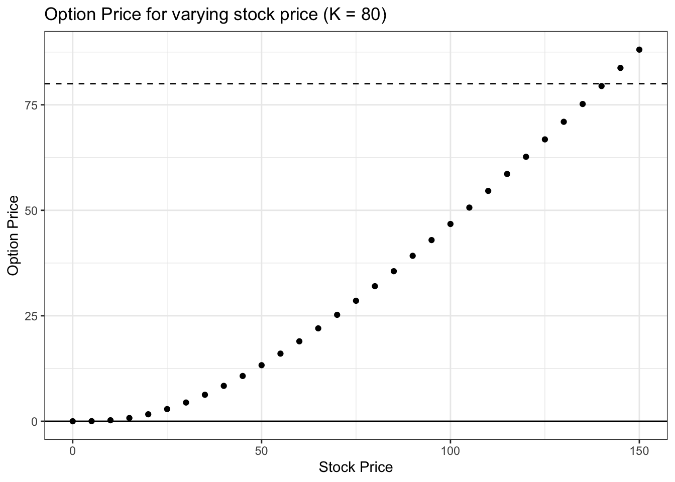
There are a couple of interesting things to note from the above chart. First, naturally, as we predicted, the option price increases with the stock price. Second, note that for very low values of the stock, the option is worth essentially zero; intuitively, this is because if the stock price is low enough, there is basically no chance that it ends up in the money and thus we exercise (so the option expires worthless). Finally, note that the option price is \(\$88.08\) when the stock price is \(\$150\) (try tail(data, 1) to see this value). This value seems high. Even if the option expired today, one would buy the stock for the strike price of 80 dollars, sell it for the market price of 150 dollars and make 70 dollars; why would the option, then, be worth \(\$18.08\) more than this \(\$70\) profit? The idea here is that (as we saw at the beginning of this chapter), because there is plenty of time left before expiry (100 days) and there is more upside than downside (the stock can go very high, and the increase in value for the option is unbounded, but even if the stock falls to zero, the option can’t be worth anything less than zero dollars; the downside is bounded), the option is valued more than what we would make if the option expired right now.
It is also important to note the slope of this line; it starts out as convex (second derivative is positive) but looks more linear for large values of S (this would continue if we had even larger values of S). This is because, once the stock price gets sufficiently above the strike price, the probability of exercising the option is very high (i.e., if the stock price is 150 dollars and the strike price is 80 dollars, we are almost certainly going to exercise because we don’t expect the stock price to fall all the way back to below 80 in the time remaining). Therefore, each additional dollar in the stock price S doesn’t really change the probability of exercising (changes in the probability of exercising create the convexity for lower values of S along the curve), and thus each dollar increase in stock price corresponds to the same increase in option price.
Let’s continue in this thread but instead vary the time to expiry for the option:
# initialize parameters
S <- 90
K <- 80
r <- .01
sigma <- 2
time <- seq(from = 1, to = 365, by = 5) / 365

# generate prices
price <- sapply(time, function(x) FUN_blackscholes(S = S, r = r,
                                       time = x, sigma = sigma, k = k))
# visualize
data <- data.table(time = time,
                   price = price)

ggplot(data, aes(x = time, y = price)) +
  geom_point() +
  theme_bw() +
  xlab("Time Until Expiry (years)") + ylab("Option Price") +
  ggtitle("Option Price for varying time to expiry (K = 80, S = 90)") +
  geom_hline(yintercept = 0) + geom_hline(yintercept = S)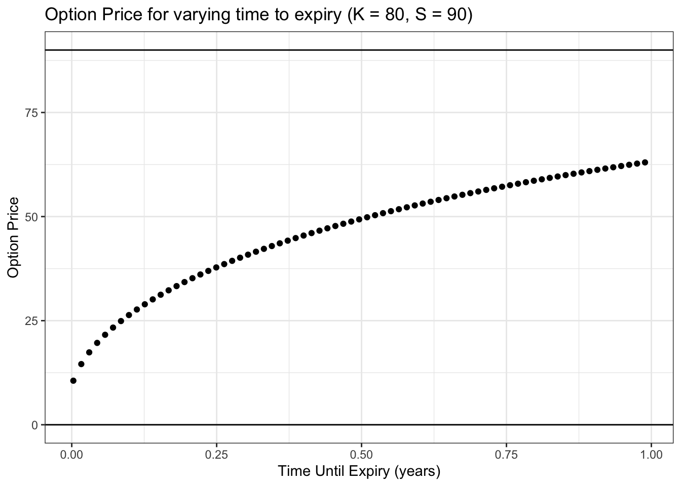
First, we can note the earliest time point here: 1 day until expiry. The option price in this case is \(\$10.58\) (try head(data, 1) to see this value), which is very close to the stock price of 90 dollars minus the strike price of 80 dollars. This makes sense; we are only one day away from expiry, so the stock doesn’t have time to move that much, and thus won’t be very far from where it sits now at 90 dollars. If it expires at 90 dollars, we make 10 dollars, because we exercise the option, buy the stock for 80 dollars and sell it for 90 dollars. Note that the option price is slightly more than 10 dollars (58 cents more, to be exact), which is for the same reason discussed above: even though we don’t expect the stock to move that much, if it does move a lot, there is more upside than downside (option value upside theoretically unbounded while downside is capped).
In general, notice the upward sloping trend. This means that, all else equal, an option that has a longer time until expiry is more valuable. This makes sense: like we’ve been talking about, options have unlimited upside but limited downside, so the more time that the stock has to move around, the higher value the option should be! Ultimately, uncertainty is good for call options, and more time until expiry introduces more uncertainty.
In financial terms, practitioners call this ‘time’ value theta. Since, all else equal, lower time values mean lower option prices, we will often observe option prices fall each day (the time until expiry reduces each day, since the expiry stays fixed); this is called theta decay.
Let’s now vary the volatility term (remember, this is taken as a given input for each stock):
# initialize parameters
S <- 90
K <- 80
r <- .01
sigma <- seq(from = .01, to = 20, by = .5)
time <- 50 / 365

# generate prices
price <- sapply(sigma, function(x) FUN_blackscholes(S = S, r = r,
                                       time = time, sigma = x, k = k))
# visualize
data <- data.table(sigma = sigma,
                   price = price)

ggplot(data, aes(x = sigma, y = price)) +
  geom_point() +
  theme_bw() +
  xlab("Stock Volatility") + ylab("Option Price") +
  ggtitle("Option Price for varying volatility (K = 80, S = 90)") +
  geom_hline(yintercept = 0) + geom_hline(yintercept = S)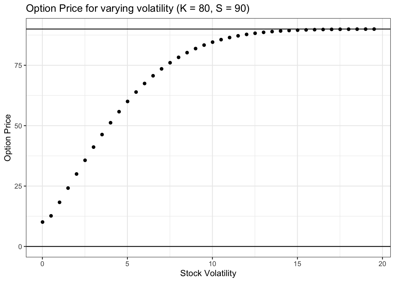
Similar to how we saw that more time until expiry increases option value, more stock volatility also increases option value. The reasoning here is the same: more uncertainty is good for option value, and more volatility in the stock is, by definition, more uncertainty.
Note that, for low values of sigma, the value of the option is very close to 10 dollars, which again is the stock price of 80 dollars minus the strike price of 70 dollars. Again, this is because, if a stock has very low volatility, we don’t expect it to move much between now and expiry; by the time we get to expiry, then, if the stock has indeed not moved much from 90 dollars, the option is worth 90 dollars minus the 80 dollar strike price (again, the option today is worth slightly more because of the unlimited upside vs. the capped downside).
Finally, note that when sigma gets very large, the option price begins to approach the stock price of 90 dollars. This is a bit tricky. If the volatility (sigma value) for the stock is extremely large, and we know that the stock has a lower bound of zero, then there is a high probability of getting a very large value for the stock at expiry (the stock will move around a ton, and has a lower bound of zero). If the stock has a very, very large value, then, at expiry, the value of the option is essentially just the value of the stock (of course, the value will be the stock price minus the strike price, but if the stock price is extremely large, the strike price is just a small fraction of the stock price). Therefore, if at expiry the option value is just equal to the stock value, then we should just price the option today at the same price as the stock. That is, if at expiry the option will just be worth the same value as the stock, then the price of the option now should just be the price of the stock now (they are equivalent!).
Finally, let’s vary the last parameter, the risk free rate:
# initialize parameters
S <- 90
K <- 80
r <- seq(from = 0, to = 5, by = .1)
sigma <- .1
time <- 100 / 365

# generate prices
price <- sapply(r, function(x) FUN_blackscholes(S = S, r = x,
                                       time = time, sigma = sigma, k = k))
# visualize
data <- data.table(r = r,
                   price = price)

ggplot(data, aes(x = r, y = price)) +
  geom_point() +
  theme_bw() +
  xlab("Risk Free Rate") + ylab("Option Price") +
  ggtitle("Option Price for varying risk free rate (K = 80, S = 90)") +
  geom_hline(yintercept = 0)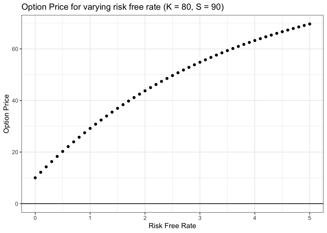
This relationship is tricky: why does option price increase with the risk free rate? Here, we can recall that if we do end up exercising the option, we have to pay the strike price K to buy the option. Imagine, now, how low the present value of the strike price K is if the risk free rate is really high. Alternatively, note that, if the risk free rate is extremely high, one could invest a small amount (say, a dollar) today and earn back a much higher amount (say, 80 dollars) by the time of expiry (of course, this is mostly theoretical; risk free rates would have to be extremely high to achieve this growth, almost certainly far higher than anything we will ever see in the real world; still it helps to get our intuition around it!). Therefore, the strike price that we will have to pay in the future (if the stock ends up above the strike price) is essentially worth nothing today (if the risk free rate is sufficiently high); that means that, as the risk free rate rises, we can buy the stock for less money (the value of K in present dollars gets lower and lower as the risk free rate rises). Buying the stock for less money (in present dollars) is good, of course, which means that the option price rises with the risk free rate!
We work through the intuition behind Black-Scholes in this video:
Click here to watch this video in your browser