Chapter 4 Random Walks
A walk?" said Catharine. “One foot in front of the other,” said Newt, “through leaves, over bridges—”
Kurt Vonnegut (Long Walk to Forever)

Motivation
Now that we have a handle on what a stochastic process actually is, let’s explore this crucial class of processes, both analytically and via simulation in R. We can use the key attributes and topics that we learned in the last chapter to solidify our frame of reference.
4.1 Gaussian Random Walk
Let’s start with a simple stochastic process that we’ve already met: a Gaussian Random Walk, which is essentially a series of i.i.d. \(N(0, 1)\) random variables through time:
\[X_0 = 0\] \[X_t = X_{t - 1} + \epsilon_t\]
Where \(t = 1, 2, ...\) and \(\epsilon_t\) is a series of i.i.d. \(N(0, 1)\) random variables.
Let’s investigate the Gaussian Random Walk further with some of the properties we’ve learned about.
# replicate
set.seed(0)

# generate a Gaussian Random Walk
data <- data.table(t = c(0, seq(from = 1, to = 100, by = 1)),
                   replicate(c(0, cumsum(rnorm(100))), n = 100))
data <- melt(data, id.vars = "t")

ggplot(data, aes(x = t, y = value, col = variable)) +
  geom_line() +
  ggtitle("100 Simulations of a Gaussian Random Walk") +
  theme_bw() +
  theme(legend.position = "none") +
  xlab("t") + ylab("X_t") +
  geom_hline(yintercept = 0)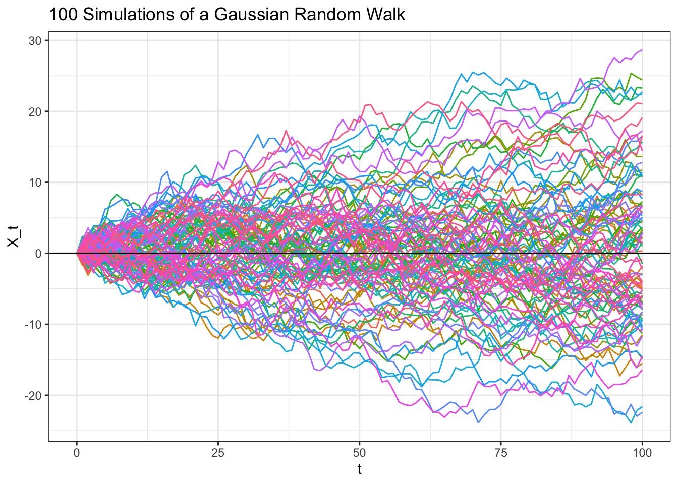
4.1.1 Strong Stationarity
Remember, a stochastic process is strongly stationary if:
\[F_{t_1, t_2, ..., t_n} = F_{t_1 + k, t_2 + k, ..., t_n + k}\]
For all \(k\), \(n\) and sets of time intervals \(t_1, t_2, ...\) in the stochastic process. Colloquially, the distributional properties of the process don’t change over time.
Let’s start with a simple case. Is \(F_{t_{1}}\) equal to \(F_{t_{5}}\), for example?
We can start by expanding \(X_t\). We have that, by definition:
\[X_t = X_{t - 1} + \epsilon_t\]
Plugging in for \(X_{t-1}\), we have:
\[X_{t - 2} + \epsilon_{t - 1} + \epsilon_t\]
Continuing in this way until we get to \(X_0 = 0\), we have:
\[X_0 + \epsilon_1 + ... + \epsilon_{t - 1} + \epsilon_t\]
Or just:
\[\epsilon_1 + ... + \epsilon_{t - 1} + \epsilon_t\]
Since each \(\epsilon\) is a Normal random variable (each i.i.d. with expectation \(0\) and variance \(1\)), and the sum of Normals is Normal, we have:
\[X_t \sim N(0, t)\]
Note that this is a similar construct to our Brownian motion; the difference is that the Gaussian Random Walk is only defined on discrete points (specifically, \(0, 1, 2...\)) where the Brownian Motion is continuous (defined for \(t \geq 0\)). This result is also intuitive given the shape of the many paths for the Gaussian Random Walk that we sampled. Scroll up to the graph above and imagine taking vertical cross sections (draw a vertical line and look at the distribution of the path intersections). The variance of these intersections grows with time (this is the variance \(t\) at play) while the mean stays at zero (as above, \(X_t\) has a mean of \(0\)).
Anyways, that means that \(F_{t_{1}}\) is the CDF of a \(N(0, 1)\) random variable, while \(F_{t_{5}}\) is the CDF of a \(N(0, 5)\) random variable. These are different CDFs (even though the structure is the same, the variance term is different) and thus the Gaussian Random Walk is not strictly stationary (intuitively, the distribution changes over time because the variance increases).
4.1.2 Weak Stationarity
Recall that a process is weakly stationary if these three conditions are satisfied:
- The mean of the process is constant. That is, \(E(X_t) = \mu\) (where \(\mu\) is some constant) for all values of \(t\).
- The second moment of \(X_t\), or \(E(X_t ^ 2)\), is finite.
- We have:
\[Cov(X_{t_1}, X_{t_2}) = Cov(X_{t_1 - k}, X_{t_2 - k})\]
For all sets of \(t_1, t_2\) and all values of \(k\).
Let’s investigate these conditions for the Gaussian Random Walk.
- First, we can calculate the expectation using a similar expansion to our exercise above. Plugging in for \(X_t\), we have:
\[E(X_t) = E(X_{t - 1} + \epsilon_t)\]
Plugging in again for \(X_{t - 1}\), we have:
\[E(X_t) = E(X_{t - 2} + \epsilon_{t - 1} + \epsilon_t)\]
This continues until we finally hit \(X_0\), which is simply \(0\). We have:
\[E(X_t) = E(X_0 + \epsilon_1 + ... + \epsilon_{t - 1} + \epsilon_t)\]
And since each \(\epsilon_t\) is i.i.d. \(N(0, 1)\), this all simply reduces to \(0\). Therefore, the expectation is indeed constant at zero (yes, it’s true that we already showed this, but it can’t hurt to explore the derivation again!).
- We have already shown that \(E(X_t) = 0\), so we have:
\[Var(X_t) = E(X^2)\]
Since \(E(X_t) ^ 2 = 0\). Since each step in the process is i.i.d., we can easily calculate the variance with a similar approach to the expectation. Plugging in our full expansion of \(X_t\), we have:
\[Var(X_t) = Var(X_0 + \epsilon_1 + ... + \epsilon_{t - 1} + \epsilon_t)\]
\(X_0\) is a constant and each \(\epsilon\) term has a variance of 1, so this reduces to:
\[Var(X_t) = E(X^2) = t\]
Of course, we could have just used the fact that \(X_t \sim N(0, t)\), as shown above, instead of solving the variance in expectation in these first two parts; however, the practice is good!
Anyways, we have shown the second moment to be finite!
- We already saw that the variance of this process is not constant. Let’s consider the covariance:
\[Cov(X_{t - k}, X_t)\]
We can use this key property of covariance…
\[Cov(X + Y, Z) = Cov(X, Z) + Cov(Y, Z)\]
…to solve this problem. Let’s use the expansion for \(X_t\) that we have employed to great success thus far:
\[Cov(X_{t - k}, X_t) =\] \[Cov(X_0 + \epsilon_1 + ... + \epsilon_{t - k}, X_0 + \epsilon_1 + ... + \epsilon_t)\]
Remember that \(X_0 = 0\) and that a constant has no covariance, so these terms drop out. Further, since each \(\epsilon\) term is i.i.d., \(Cov(\epsilon_i, \epsilon_j) = 0\) for \(i \neq j\). We are just left, then, with:
\[Cov(\epsilon_1, \epsilon_1) + Cov(\epsilon_2, \epsilon_2) + ... + Cov(\epsilon_{t - k}, \epsilon_{t - k})\] \[= Var(\epsilon_1) + Var(\epsilon_2) + ... + Var(\epsilon_{t - k})\]
And, since each variance is 1, we are simply left with:
\[Cov(X_{t - k}, X_t) = t - k\]
Since our Covariance clearly depends on \(t\) and \(k\) (the larger \(k\) is, the lower the covariance; this is intuitive because \(X_{t - k}\) is farther from \(X_t\) when \(k\) is large), we do not satisfy the third condition of weak stationary. Therefore, this Gaussian Random Walk is not weakly stationary.
4.1.3 Martingale
Recall that a stochastic process is a martingale if:
\[E(X_{n + 1} | X_1, ..., X_n) = X_n\]
For a Gaussian Random Walk, at every increment we are adding a random variable (an \(\epsilon\) term) with an expectation of \(0\). Therefore, the expectation of \(X_{n + 1}\) is just \(X_n\) (since we are adding something that we expect to be zero!).
Therefore, the Gaussian Random Walk is a martingale.
4.1.4 Markov
Recall that a stochastic process \(X_t\) is Markov if:
\[P(X_t|X_1, X_2, ..., X_{t - 1}) = P(X_t | X_{t - })\]
That is, the probability distribution of \(X_t\), given the entire history of the process up to time \(t\), only depends on \(X_{t - 1}\). As we discussed in the last chapter, a Gaussian Random Walk is Markov!
4.2 Simple Random Walk
We can continue our study of random walks with a more fundamental structure; a simple random walk \(X_t\) is a stochastic process where:
\[X_t = \sum_{i = 1}^t Y_i\]
Where \(X_0 = 0\). We let the \(Y\) random variables be i.i.d. such that \(P(Y_i = 1) = p\) and \(P(Y_i = -1) = 1 - p = q\) (that is, \(Y\) can only equal \(1\) with probability \(p\) or \(-1\) with probability \(q = 1 - p\)). We can envision, then, \(X_t\) simply moving up or down \(1\) at each time point, governed by the probability \(p\) (of moving up \(1\); remember that \(q\), or \(1 - p\), is the probability of moving down \(1\)). Let’s simulate a simple random walk to visualize its activity:
# replicate
set.seed(0)

# function to generate random walks
FUN_simplewalk <- function(t, p) {

  x <- 0
  for (i in 1:t) {
    x <- c(x, x[length(x)] + sample(c(-1, 1), 1, prob = c(1 - p, p)))
  }

  return(x)
}


# generate and visualize
data <- data.table(t = 0:100,
                   x = FUN_simplewalk(100, .6))
ggplot(data, aes(x = t, y = x)) +
  geom_line() +
  theme_bw() +
  ylab("X_t") +ggtitle("Simple Random Walk for 100 steps (p = .6)")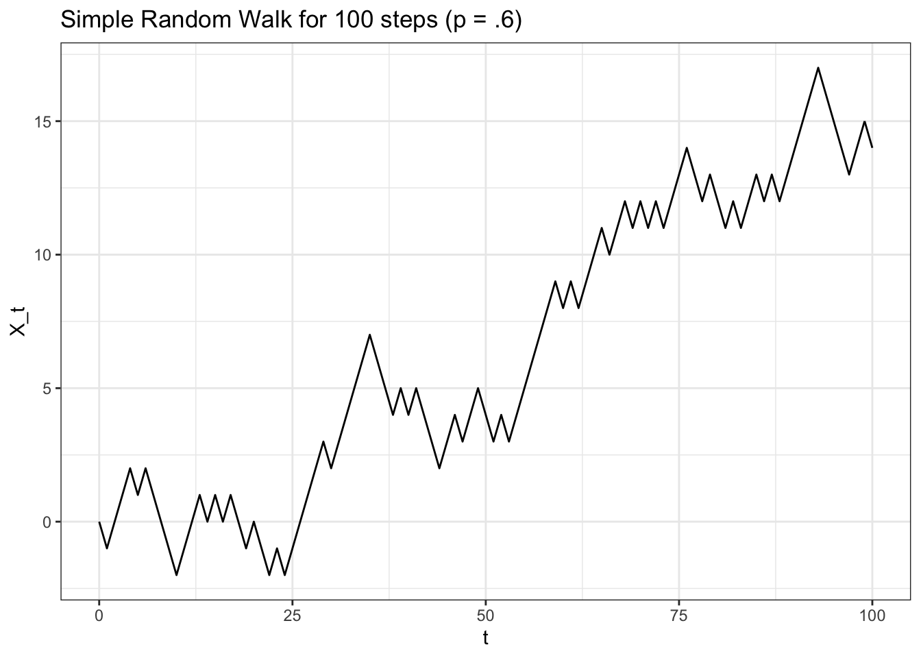
In this case, \(p = .6\), so there is no surprise that the random walk drifts upwards (most of the moves will be ‘up moves!’). A symmetric simple random walk is one where, well, \(p = .5\), so that we have symmetric probabilities of moving up or down.
We can easily calculate some of the key metrics of \(X_t\). Let’s start with the expectation (remember that \(X_0 = 0\)):
\[E(X_t) = E(X_0 + Y_1 + Y_2 + ... + Y_n)\] \[ = E(Y_1) + E(Y_2) + ... + E(Y_n)\]
Remember that each \(Y_i\) term is i.i.d. with probability \(p\) of taking on the value of \(1\) and probability \(1 - p\) of taking on the value \(-1\), so the expectation of each \(Y_i\) term is:
\[E(Y_i) = p \cdot 1 + (1 - p) \cdot (-1)\]
\[= p + p - 1 = 2p - 1\]
Plugging in to \(E(X_t)\) above:
\[E(X_t) = t(2p - 1)\]
This expectation is intuitive: if \(p = 1/2\), then \(E(X_t) = 0\), which makes sense by symmetry (if the random walk is equally likely to go up or down, then we expect it to not move in the long run!). If we have \(p > 1/2\), then \(E(X_t) > 0\), which makes sense because the random walk ‘drifts’ upwards as we saw above (and, of course, for \(p < 1/2\), we have \(E(X_t) < 0\) for the same reason).
We can also calculate the variance:
\[Var(X_t) = Var(Y_1 + Y_2 + ... + Y_n)\]
\[Var(X_t) = Var(Y_1) + Var(Y_2) + ... + Var(Y_n)\]
We can add the variances because each \(Y_i\) term is i.i.d. We can find the variance of \(Y_i\) by using the following relation:
\[Var(Y_i) = E(Y_i^2) - \big(E(Y_i)\big)^2\]
We already have \(E(Y_i)\), and can calculate \(E(Y_i^2)\) by simply looking at the structure of \(Y_i^2\). Since \(Y_i\) only takes on values \(1\) and \(-1\), we have that \(Y_i^2\) will always take on the value 1. We therefore have, plugging in \(E(Y_i) = 2p - 1\) from before:
\[Var(Y_i) = 1 - (2p - 1)^2\]
\[= 1 - (4p^2 - 4p + 1)\] \[= 1 - 4p^2 + 4p - 1\] \[=4p - 4p^2\] \[=4p(1 - p)\]
Which means that the variance of \(X_t\) is simply \(t2p(2 - p)\).
Let’s check our expectation and variance by simulating many paths of simple random walks:
# replicate
set.seed(0)

# define parameters and generate results
p <- .55
t <- 100
results <- replicate(FUN_simplewalk(t = t, p = p), n = 1000)
results <- results[t + 1, ]

# expectations should match
t * (2 * p - 1); mean(results)
## [1] 10## [1] 9.826# variances should match
t * 4 * p * (1 - p); var(results)## [1] 99## [1] 94.61234Our analytically results look close to the simulated results!
4.2.1 Properties
We can almost immediately say that the simple random walk is not strongly stationary because of a similar argument to the Gaussian random walk above: the variance that we calculated above is a function of \(t\) and thus increases with time, meaning that the distribution of \(X_5\) will be different, than, say, the distribution of \(X_{17}\) (we have that \(Var(X_{17}) > Var(X_5)\)).
Further, we can use a similar approach as before to show that the simple random walk is also not weakly stationary. Consider the covariance:
\[Cov(X_{t - k}, X_t)\]
Plugging in that each \(X_t\) is a sum of \(Y_i\) random variables:
\[=Cov(Y_1 + ... + Y_{t - k}, Y_1 + ... + Y_t)\]
Since the \(Y_i\) terms are all i.i.d., using the property from above (scroll to the Gaussian random walk weak stationarity exercise for more elaboration) we have:
\[= Var(Y_1) + Var(Y_2) + Var(Y_{t - k})\]
Again, each \(Y_i\) term has the same variance (the terms are i.i.d.), so we have:
\[= (t - k) Var(Y_1)\]
Therefore, because the covariance clearly depends on \(t\) (we multiply by \(t - k\)), this process is not weakly stationary.
Let’s perform the crucial calculation to determine if \(X_t\) is a martingale; that is, if this condition holds:
\[E(X_{t + 1} | X_1, ..., X_t) = X_t\]
We can calculate the conditional expectation:
\[E(X_{t + 1} | X_t) = X_t + 1 \cdot p - 1 \cdot(1 - p)\]
Since, conditioned on \(X_t\), we either move up \(1\) with probability \(p\) or down \(1\) with probability \(1 - p\). This only equals \(X_t\) if \(p - (1 - p) = 2p - 1 = 0\), which is only the case if \(p = 1/2\). Therefore, \(X_t\) is a martingale only if we have \(p = 1/2\). This makes sense; we only expect a move of zero if we have symmetric probabilities of moving up and down (otherwise we have drift up or down).
Finally, we can see that a simple random walk is Markov; for the distribution of \(X_t\), we have that \(X_{t - 1}\) provides all of the information from the history of \(X_t\) that we need. Similar to the Gaussian random walk, as long as we know where we were on the previous step, it doesn’t matter how we got there; our distribution for the next step is still the same.
4.2.2 Barriers
We’ve been dealing with unrestricted simple random walks where, as the name implies, there are no limits to where the random walk goes! We can add barrier that either ‘absorb’ or ‘reflect’ the random walk.
If a random walk hits an absorbing barrier it is, well, absorbed. The random walk finishes and the process sits at that absorbing barrier for the rest of time. Formally, if \(a\) is an absorbing barrier, and \(X_t\) hits \(a\) for the first time at time \(k\), then \(X_t = a\) for \(t \geq k\) with probability \(1\).
Random walks with absorbing barriers are still not weakly stationary or strongly stationary (for essentially the same reasons that unrestricted random walks are not weakly stationary or strongly stationary). Random walks with absorbing barriers are still Markov and still Martingale: even if we are trapped in the absorbing state, the Markov property holds (we know where we will be in the next step, so conditioning on the entire history of the process gives no more information than conditioning on just the previous step), and the process is still a Martingale (the expected value of the next step is just the current step, because we know that the next step will be the current step; we are in the absorbing state!).
If the random walk hits a reflecting barrier it is, well, reflected. The random walk ‘bounces’ back from the barrier to the value below (or above) the barrier. For example, if \(r_{up}\) is an upper reflecting barrier and \(r_{down}\) is a lower reflecting variable, then for any \(X_t = r_{up}\) (whenever we hit the upper reflecting barrier) we have \(X_{t + 1} = r_{up} - 1\) with probability \(1\), and similarly for any \(X_t = r_{down}\) we have \(X_{t + 1} = r_{down} + 1\) with probability \(1\).
Again, reflecting barriers are still not weakly stationary or strongly stationary (for, again, much the same reasons). They are still Markov, since, even if we are at the reflecting barrier, the most recent value in the process gives us as much information as the entire history of the process. These random walks are not Martingales, though, since if we are the reflecting barrier, we know that the next value will be different from the value that we are currently at.
4.2.3 Behavior
Some key questions arise naturally when we consider random walks (in this section, we will be discussing unrestricted simple random walks unless otherwise specified). For example, one might ask what the probability is of the random walk ever reaching a certain value. For example, if we have a simple random walk with \(p = .6\), what is the probability that the random walk ever hits \(-10\)? We know that the random walk with drift upwards as time passes, but will it hit \(-10\) first?
Let’s define \(P_k\) as the probability that a random walk ever reaches the value \(k\). We have:
\[P_k = P_1^k\]
That is, the probability that the random walk ever reaches \(k\) is just the probability that the random walk ever reaches \(1\), to the power of \(k\). This makes sense, because we can think of getting to \(k\) as essentially getting to \(1\) (which has probability \(P_1\)), but \(k\) times. Since each step in the random walk is independent, we can simply raise the probability to the power of \(k\).
We can focus, then, on finding \(P_1\). In this case, it will be useful to employ first step analysis, or conditioning on the first step in the random walk and working out our probability from there. More formally:
\[P_1 = p P_1|U + qP_1 | D\]
Where \(P_1|U\) is the probability of reaching \(1\) given that the first step in the random walk is an ‘Up’ move and \(P_1|D\) is the probability of reaching \(1\) given that the first step in the random walk is a ‘Down’ move. This becomes:
\[P_1 = p + qP_2\]
Since if we move up on the first move then we are at \(1\), and thus the probability of hitting \(1\) is, well, \(1\). If we move down on the first move, then the probability of hitting \(1\) is now \(P_2\), because we have to go up \(2\) (from \(-1\)) to hit \(1\) now! We can plug in \(P_1^2\) for \(P_2\) using our equation above, which gives:
\[P_1 = p + qP_1^2\]
\[qP_1 ^ 2 - P_1 + p = 0\]
We can find roots with the quadratic equation:
\[\frac{1 \pm \sqrt{1 - 4qp}}{2q}\]
The \(\sqrt{1 - 4pq}\) term is a bit tough to work with, so we will use a little trick. We know that \(1 = p + q\), and thus \(1^2 = 1 = (p + q)^2 = p^2 + q^2 + 2pq\). If we take:
\[1 = p^2 + q^2 + 2pq\]
And subtract \(4pq\) from both sides, we get:
\[1 - 4pq = p^2 + q^2 - 2pq\]
So, we can just plug in \(p^2 + q^2 - 2pq\) for \(1 - 4pq\), and this nicely factors to \((p - q)^2\) (technically, the square root of \((p - q)^2\) is \(|p - q|\), since just \(p - q\) can be negative and the square root of something can’t be negative; we won’t have to worry about that in this case, though, as you will see). We are left with:
\[\frac{1 + \pm p - q}{2q}\]
In the \(+\) case, we have:
\[\frac{1 + p - 1 + p}{2q} = \frac{2p}{2q} = \frac{p}{q}\]
In the \(-\) case, we have:
\[\frac{1 - p + 1 - p}{2q} = \frac{2q}{2q} = 1\]
So our two roots are \(\frac{p}{q}\) and \(1\). In our case, when we have \(p > q\), we will use \(1\) as our root (since \(\frac{p}{q} > 1\) in this case; this is why we didn’t have to worry about the absolute value earlier!). The \(\frac{p}{q}\) makes sense; the lower that \(p\) gets, the lower the probability of hitting \(1\) gets.
So, we found that \(P_1 = \frac{p}{q}\) when \(p < q\) and \(P_1 = 1\) when \(p \leq 1/2\). Using \(P_k = P_1^k\), we simply have \(P_k = (\frac{p}{q})^k\) when \(p < q\) and \(P_k = 1\) when \(p \leq 1/2\) for \(k > 0\). That is, we will definitely hit \(k\) if \(p\geq 1/2\), whereas we might hit \(k\) if \(p < 1/2\) (with probability \((\frac{p}{q})^k\), which is less than \(1\)).
Note that this result is symmetric to the downside; that is, \(P_k\) for \(k < 0\) is \((\frac{q}{p})^k\) for \(p > 1/2\) and \(1\) for \(p \leq 1/2\). Also note that this gives an interesting result: if \(p = 1/2\), then the probability that the random walk hits any value is \(1\); that is, we are certain that the random walk will hit all values eventually!
Let’s test this probability with a simulation with \(p = .3\), where the probability of hitting, say, \(2\) is \((\frac{.3}{.7})^2 = .184\). Naturally, we can’t let our simulation run forever; we’ll just let the random walk run long enough so that, if it hasn’t hit \(2\) by that point, it probably never will (it likely will be far enough on the negative side of \(0\) that it will never climb back up to \(2\)).
# replicate
set.seed(0)

# define parameters and generate results
p <- .3
t <- 75
results <- replicate(FUN_simplewalk(t = t, p = p), n = 100)

# how many get above 2?
mean(apply(results, 2, max) >= 2)
## [1] 0.19# visualize
data <- data.table(t = 1:(t + 1),
results)
data <- melt(data, id.vars = "t")
ggplot(data, aes(x = t, y = value, col = variable)) +
geom_line(alpha = 1 / 4) +
theme_bw() + theme(legend.position = "none") +
geom_hline(yintercept = 2, linetype = "dashed") +
geom_hline(yintercept = 0) +
xlab("t") + ylab("X_t") +
ggtitle("How many random walks hit 2 for p = .6?")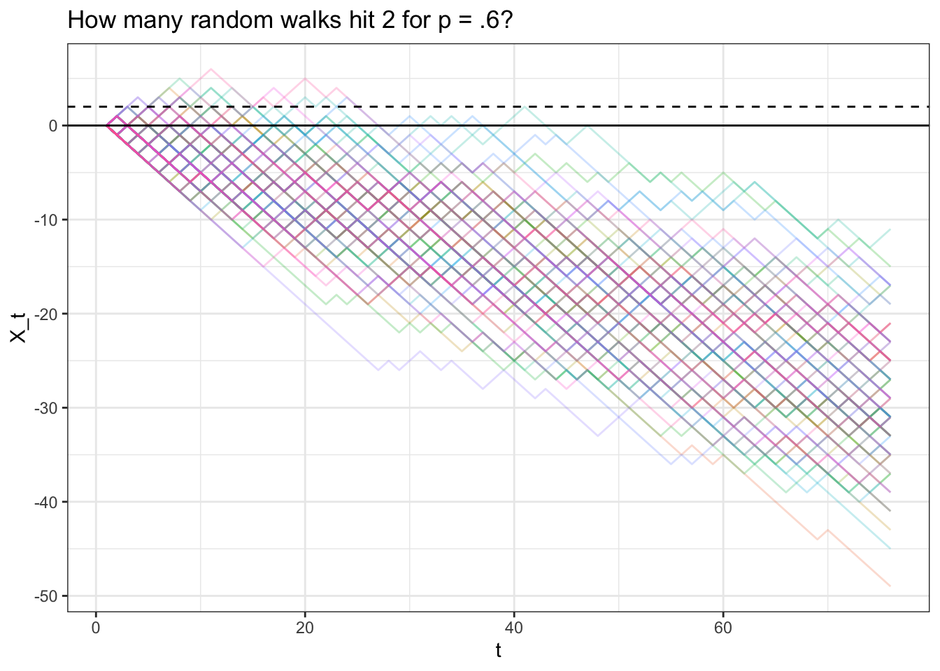
We see that .19 of the simulations hit \(2\), which is close to our analytically result!
Here’s a video walkthrough of this type of problem:
Click here to watch this video in your browser
Finally, now that we have a handle on the probability of hitting a certain value, let’s try to find the expected time until we hit a specific value. Let’s define \(T_k\) as the amount of time it takes to go from \(0\) to \(k\) (where \(k > 0\)) for a simple, unrestricted random walk. We are interested in \(E(T_k)\), which we can luckily split into simpler terms:
\[E(T_k) = E(T_1) + E(T_1) + ... E(T_1) = kE(T_1)\]
This equation holds because we can think of going up to the value \(k\) as just going up to the value \(1\), but \(k\) times (to clarify, we don’t mean hitting \(1\) a total of \(k\) times, but hitting \(1\), then \(2\), etc. until we are up to \(k\)).
Let’s use first step analysis again to try to find \(E(T_1)\):
\[E(T_1) = 1 + p\cdot 0 + qE(T_2) = 1 + 2q E(T_1)\]
The \(1\) comes from, well, taking the first step. The \(p \cdot 0\) term is when the random walk goes up one step with probability \(p\), hits \(1\) and thus has \(0\) more time expected until it hits \(1\). Finally, we have \(E(T_2) = 2E(T_1)\) from our previous equation.
We’re thus left to solve the equation:
\[E(T_1) = 1 + 2q E(T_1)\]
Let’s start with the case where \(p < q\). We know from the previous section that, if \(p < q\), the probability of ever hitting \(1\) is \(\frac{p}{q} < 1\). That means that, with some non-zero probability (specifically, \(1 - \frac{p}{q}\)), the process will never hit \(1\), and thus take an infinite amount of time (because it will never hit \(1\)). Therefore, since there is a nonzero probability of an infinite waiting time, the expectation of the waiting time is simply \(\infty\) (think about it: when we perform the calculation for expectation, we will have some non-zero probability times \(\infty\), which is just \(\infty\)).
When \(p = 1/2\), we simply have:
\[E(T_1) = 1 + E(T_1)\]
Which, of course, means that \(E(T_1)\) is again \(\infty\), since if you add \(1\) to \(\infty\) you get \(\infty\).
Finally, if \(p > q\), we get:
\[E(T_1) = 1 + 2q E(T_1)\]
\[E(T_1) - 2qE(T_1) = 1\]
\[E(T_1)(1 - 2q) = 1\] \[E(T_1) = \frac{1}{1 - 2q}\]
We have: \[1 - 2q = 1 - 2(1 - p) = 1 - 2 + 2p = p + p - 1 = p - q\]
Plugging this in, we get:
\[E(T_1) = \frac{1}{p - q}\]
So, therefore, if we recall that \(E(T_k) = kE(T_1)\), we have that when \(p \leq 1/2\), \(E(T_k) = \infty\) for \(k > 0\) and when \(p > q\) we have \(E(T_k) = \frac{k}{p - q}\).
Let’s simulate a bunch of paths and see if this expectation makes sense. We will try \(k = 5\) and \(p = .55\) which, according to \(E(T_k) = \frac{k}{p - q}\), should have an expected ‘hitting time’ of \(\frac{5}{.55 - .45} = 50\).
# replicate
set.seed(0)

# define parameters and generate results
p <- .55
t <- 500
results <- replicate(FUN_simplewalk(t = t, p = p), n = 100)


# see how long it took to get to 5
results_exp <- apply(results, 2, function(x) {

    # hit 5
    if (max(x) >= 5) {
      return(min(which(x == 5)) - 1)
    }

    return(502)
  })

# should match
5 / (p - (1 - p)); mean(results_exp)
## [1] 50## [1] 49.48# stop all the results after it hits 5
for (i in 1:ncol(results)) {
results[(results_exp[i] + 2):nrow(results), i] <- -10000
}
# visualize
data <- data.table(t = 1:(t + 1),
results)
data <- melt(data, id.vars = "t")
data <- data[value > -10000]
ggplot(data, aes(x = t, y = value, col = variable)) +
geom_line(alpha = 1 / 4) +
theme_bw() + theme(legend.position = "none") +
geom_hline(yintercept = 5, linetype = "dashed") +
geom_hline(yintercept = 0) +
geom_vline(xintercept = 50) +
xlab("t") + ylab("X_t") +
ggtitle("How long until we hit 5 for p = .55?")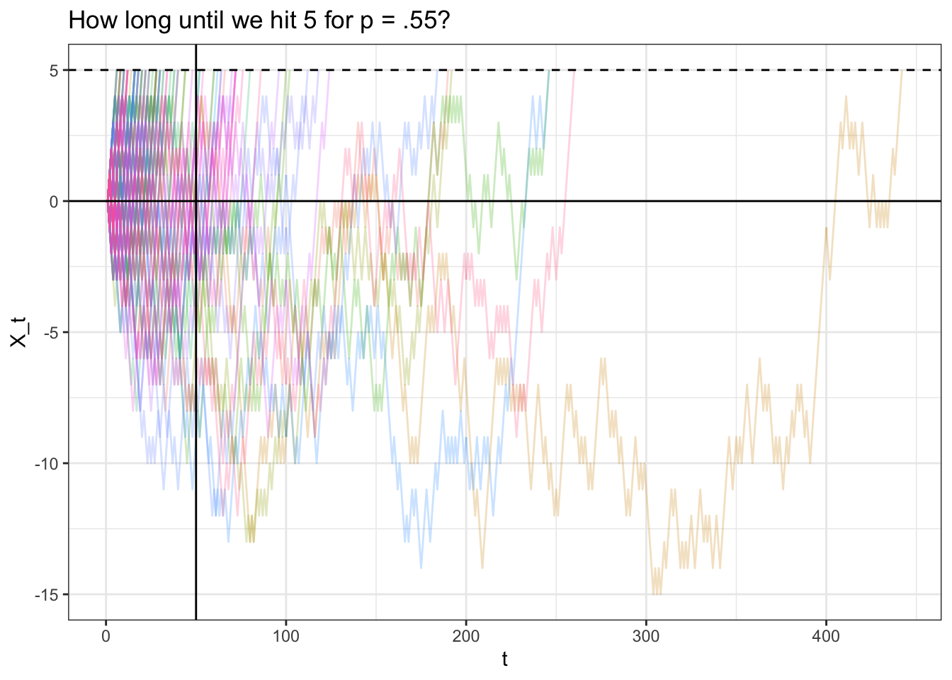
Note that our analytically result is very close to our empirical result of 49.48. The chart seems ‘right-skewed’; many of the paths hit \(5\) long after \(t = 50\), but most of the paths are clustered to the left of \(t = 50\) (they hit \(5\) well before \(t = 50\)); this balances out to a mean of \(50\).
Finally, here’s a video walkthrough of this topic:
Click here to watch this video in your browser
4.3 Gambler’s Ruin
Let’s turn to a popular random walk, accurately titled ‘the Gambler’s Ruin’; this problem will help us to explore absorbing barriers and how they affect the behavior of random walks.
We have two gamblers, named simply \(A\) and \(B\). There are \(N\) total dollars in the game; let \(A\) start with \(j\) dollars, which means \(B\) starts with \(N - j\) dollars.
The Gamblers play repeated, one round games. Each round, \(A\) wins with probability \(p\), and \(B\) wins with probability \(1 - p\), which we will label as \(q\) (the rounds are independent). If \(A\) wins, \(B\) gives one dollar to \(A\), and if \(B\) wins, \(A\) gives one dollar to \(B\). The game ends when one of the gamblers is ruined (they get to zero dollars), which means that the other gambler has all of the \(N\) dollars.
Let’s play a simple game with 10 dollars (\(N = 10\)) where \(A\) has the slight edge in each game \(p = .6\) and both players start with 5 dollars:
# replicate
set.seed(0)

FUN_ruin <- function(p, N, j) {

  # loop
  while (TRUE) {


    # break condition
    if (j[length(j)] == N || j[length(j)] == 0) {
      return(j)
    }

    # iterate
    const_play <- rbinom(1, 1, p)

    if (const_play == 1) {
      j <- c(j, j[length(j)] + 1)
    }

    if (const_play == 0) {
      j <- c(j, j[length(j)] - 1)
    }
  }
}


data <- data.table(A = FUN_ruin(p = .6, N = 10, j = 5))
data$t <- 1:nrow(data)
ggplot(data, aes(x = t, y = A)) +
  geom_line() +
  ggtitle("Gambler's Ruin") +
  theme_bw() + ylim(c(0, 10)) +
  geom_hline(yintercept = 0) +
  geom_hline(yintercept = 10)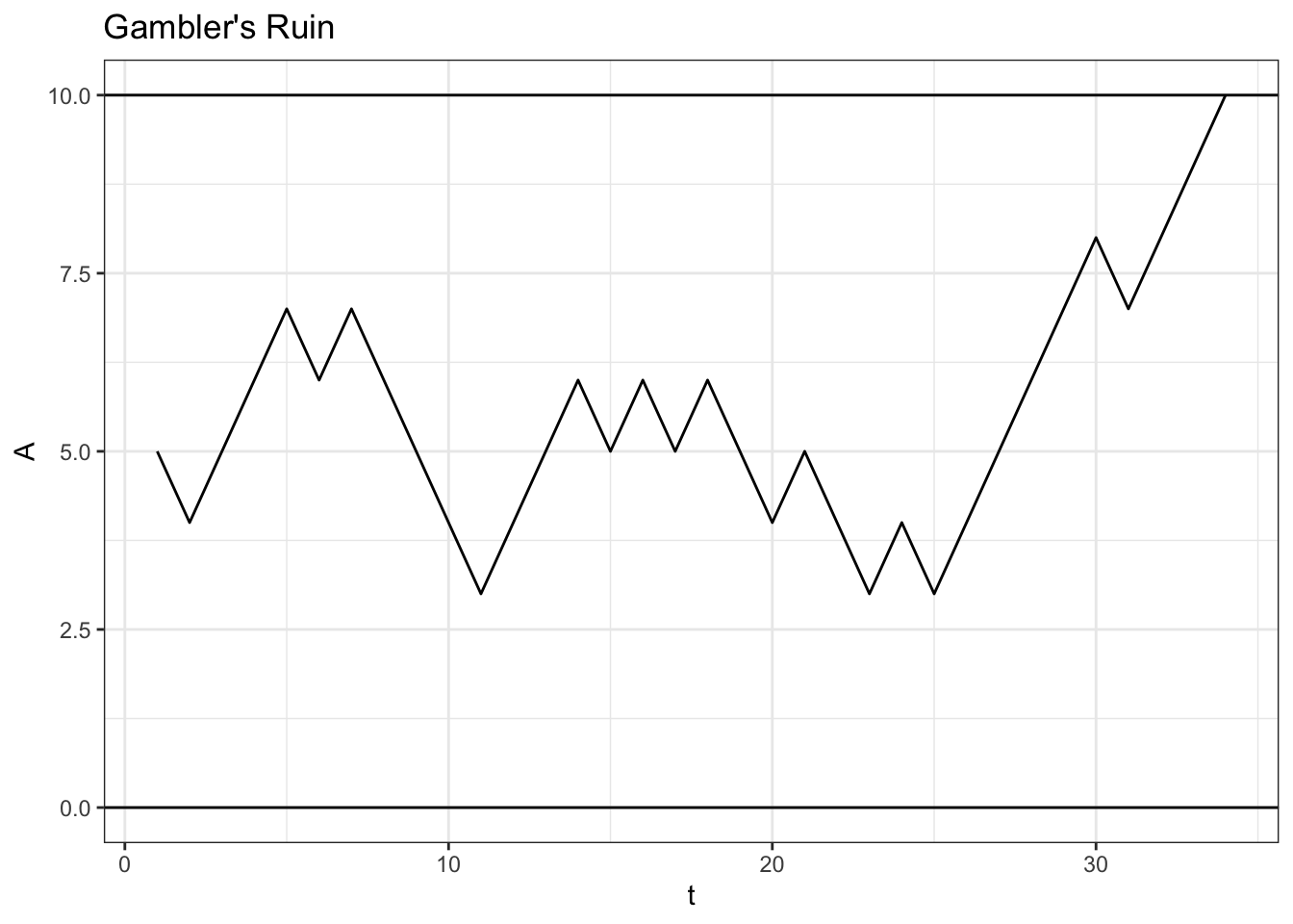
In this game, \(A\) won in the end (even though it got a little bit hairy in the middle for \(A\)!).
4.3.1 Win Probability
Naturally, some questions start to arise. Of course \(A\) had the advantage in the game above, since \(p = .6\). Does that mean \(A\) would win 60% of games? What about if we started \(A\) with less money, say 4 dollars (while \(B\) starts with 6)? Would \(A\) still be favored?
All of these thoughts boil down to a simple question: given \(p\) (the probability of \(A\) winning any one game) and \(N\) and \(j\) (the total number of dollars in the game and the total number of dollars that \(A\) starts out with) what is the probability that \(A\) wins the game and \(B\) is ‘ruined?’
Let’s use some general notation to solve this problem. We can define, for a given game (where \(N\) and \(p\) are specified), \(w_j\) as the probability that \(A\) wins given that \(A\) has \(j\) dollars. Formally:
\[w_j = P(A \; wins | A \; starts \; at \; j \; dollars)\]
With the edge conditions:
\[w_0 = 0, \; \; w_N = 1\]
Because if \(A\) has \(0\) dollars then the game is over and he has lost, by definition, and if \(A\) has \(N\) dollars then the game is over and \(A\) has won, also by definition.
Since \(A\) has probability \(p\) of winning each game (independently) we can write (again, using first step analysis and thus conditioning on the outcome of the first game):
\[w_j = p \cdot w_{j + 1} + q \cdot w_{j - 1}\]
We’re going to use a little trick here. Since \(p + q = 1\), we can plug \(p + q\) into the left hand side:
\[(p + q) \cdot w_j = p \cdot w_{j + 1} + q \cdot w_{j - 1}\]
And moving everything over:
\[0 = p \cdot w_{j + 1} - (p + q) \cdot w_j + q \cdot w_{j - 1}\]
Let’s pause here. We are going to have to make use of a ‘\(2^{nd}\) order homogeneous equation.’ We’re going to discuss the results of this tool, although we won’t solve it here, since this type of mathematical tool is a bit outside of the scope of this book.
For an equation of the form (with constants \(a\), \(b\) and \(c\)) we have:
\[aq_n + bq_{n - 1} + cq_{n - 2} = 0\]
If we write a similar equation but with \(x^n\) instead of \(q_n\):
\[ax ^ n + bx ^ {n - 1} + cx ^ {n - 2} = 0\]
Dividing both sides by \(x^{n - 2}\):
\[ax ^ 2 + bx+ c= 0\]
We can then solve for \(x\) with the quadratic formula and we will get two roots \(x_1\) and \(x_2\). Finally, this gives us:
\[q_n = c_1x_1^n + c_2x_2^n\]
Where \(c_1\) and \(c_2\) are constants. We can use the edge conditions of \(q_n\) to find these constants.
This is a very nifty result, especially since we left off at:
\[p \cdot w_{j + 1} - (p + q) \cdot w_j + q \cdot w_{j - 1} = 0\]
Following the steps laid out above, this becomes:
\[p \cdot x^2 - (p + q) x + q = 0\]
We can use the quadratic formula here:
\[\frac{(p + q) \pm \sqrt{(p + q)^2 - 4pq}}{2p}\]
We know that \(p + q = 1\), but let’s leave it as \(p + q\) for now in the numerator and expand the \((p + q) ^ 2\) term, since it may help us factor this term down:
\[=\frac{(p + q) \pm \sqrt{p^2 + q^2 + 2pq - 4pq}}{2p}\]
\[=\frac{(p + q) \pm \sqrt{p^2 + q^2 - 2pq}}{2p}\]
We have that \((p^2 + q^2 - 2pq) = (p - q)^2 = (q - p)^2\), so we can plug in:
\[=\frac{(p + q) \pm \sqrt{(p - q)^2}}{2p}\]
\[=\frac{(p + q) \pm (p - q)}{2p}\]
Remember that \(p - q = p - (1 - p) = 2p - 1\) (and \(q - p = 1 - 2p\), but the flipping of signs doesn’t matter much here because we have \(\pm\) anyways!), so we have:
\[=\frac{(p + q) \pm 2p - 1}{2p}\]
Remembering that \((p + q) = 1\), we have:
\[=\frac{1 \pm 2p - 1}{2p}\]
Which gives us the two roots \(\frac{q}{p}\) and \(1\).
Now that we have the two roots, we can move to the next step in the process outlined above:
\[w_j = c_1 1^j + c_2(\frac{q}{p})^j\]
We can use the edge conditions \(w_0 = 0\) and \(w_N = 1\). First, we have:
\[w_0 = 0 = c_1 + c_2\]
Which tells us that \(c_1 = -c_2\). Next, we have:
\[w_N = 1 = c_1 1^N + c_2(\frac{q}{p})^N\]
\[1 = c_1 + c_2 (\frac{q}{p})^N\]
Plugging in \(c_1 = -c_2\):
\[1 = -c_2 + c_2 (\frac{q}{p})^N\]
\[1 = c_2(-1 + (\frac{q}{p})^N\] \[c_2 = \frac{1}{(\frac{q}{p})^N - 1}\]
And remembering \(c_1 = -c_2\):
\[c_1 = \frac{1}{(1 - \frac{q}{p})^N}\]
Which means we are left with:
\[w_j = \frac{1}{(1 - \frac{q}{p})^N} + \big(\frac{(\frac{q}{p})^j}{(\frac{q}{p})^N - 1}\big)\]
\[= \frac{1}{(1 - \frac{q}{p})^N} - \big(\frac{(\frac{q}{p})^j}{(1 - \frac{q}{p})^N}\big)\] \[= \frac{1 - (\frac{q}{p})^j}{1 - (\frac{q}{p})^N}\]
Voila! We now have a probability, for a given \(p\), \(j\) and \(N\), that \(A\) will win!
Sharp eyed readers may note that when \(q = p\), the above equation is undefined, since the denominator is \(1 - 1 = 0\). The above derivation, therefore, just holds for \(q \neq p\).
If we have \(p = q\), then our two roots above are still \(1\) and \(\frac{q}{p} = 1\). That is, we have a double root at \(1\), which is not going to help us with our \(c_1\) and \(c_2\) equation. Here, we’re going to do a bit of mathematical hand-waving that we won’t prove (since, again, differential equations is outside of the scope of this book) and say that our equation for \(w_j\) in terms of \(c_1\) and \(c_2\) becomes:
\[w_j = c_1 \cdot j \cdot 1^j + c_21 ^j\]
\[= j c_1 + c_2\]
That is, since we have a double root at \(1\), we have that \(1\) becomes the coefficient of both \(c_1\) and \(c_2\). Note that the hand-wavy part comes with the extra \(j\) term as a coefficient for \(c_1\); this is the part that we won’t prove, since it requires an understanding of differential equations.
Anyways, carrying on as before, and using \(w_0 = 0\) and \(w_N = 1\), we have…
\[0 = 0 \cdot c_1 + c_2\] \[c_2 = 0\]
…from the first condition and…
\[1 = N c_1 + c_2\] \[\frac{1}{N} = c_1\]
…for the second condition (since \(c_2 = 0\)). That means we are just left with:
\[w_j = jc_1 = \frac{j}{N}\]
Voila! We now have the probability of \(A\) winning for some \(j\) and \(N\), when \(p = 1/2\). Note that this is intuitive; the larger that \(j\) is relative to \(N\) (i.e., the more money that \(A\) starts out with relative to the total endowment), the higher the probability that \(A\) wins (and, if \(j = N/2\), we have that \(A\) has a \(1/2\) probability of winning, which makes sense because the game is perfectly symmetric!).
Anyways, let’s investigate how this probability changes for different values of the input. First, we can fix the inputs \(N = 10\) and \(j = 5\) and vary \(p\) to see how the win probability changes:
FUN_ruinprob <- function(N, p, j) {

  # edge cases
  if (p == 0) {
    return(0)
  }

  if (p == 1) {
    return(1)
  }
  if (p == 1 / 2) {
    return(j / N)
  }

  q <- 1 - p
  return((1 - (q / p) ^ j) / (1 - (q / p) ^ N))
}

# initiate parameters and generate probabilities
N <- 10
j <- 5
p <- seq(from = 0, to = 1, by = .01)
w <- sapply(p, function(x) FUN_ruinprob(N, x, j))

# visualize
data <- data.table(p = p, w = w)
ggplot(data, aes(x = p, y = w)) +
  geom_point() +
  theme_bw() +
  ggtitle("Gambler's Ruin (N = 10, j = 5)") +
  xlab("p") + ylab("P(A Wins)")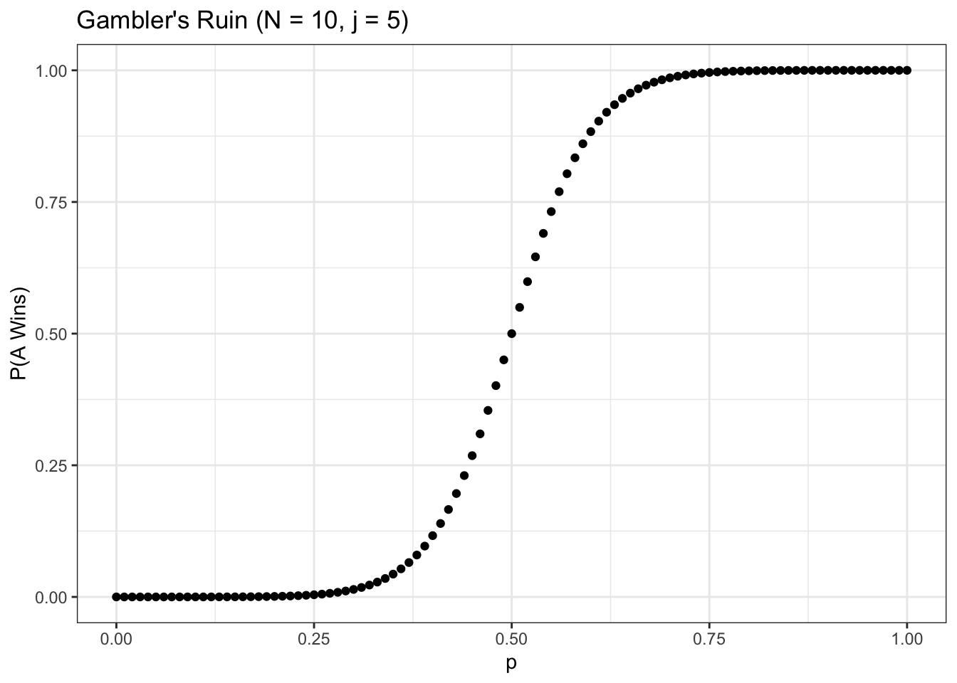
Unsurprisingly, as we increase \(p\), the probability that \(A\) wins rises rapidly (it gets very close to \(1\) for \(p \geq .75\), and symmetrically very close to \(0\) for \(p \leq .25\)). As we increase \(N\) (keeping \(j\) at \(N/2\)) the function gets even steeper:
# initiate parameters and generate probabilities
N <- 50
j <- 25
p <- seq(from = 0, to = 1, by = .01)
w <- sapply(p, function(x) FUN_ruinprob(N, x, j))

# visualize
data <- data.table(p = p, w = w)
ggplot(data, aes(x = p, y = w)) +
  geom_point() +
  theme_bw() +
  ggtitle("Gambler's Ruin (N = 50, j = 25)") +
  xlab("p") + ylab("P(A Wins)")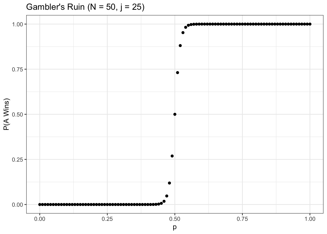
Note that, in this chart, the win probability for \(A\) goes to \(0\) or \(1\) much quicker. This is intuitive, since a larger \(N\) means that if \(A\) is the underdog (\(p < .5\)), then \(A\) is less likely to ‘pull off the upset’ because the sample space is larger (\(A\) has to ‘get lucky’ for more rounds). A game with a lower \(N\) introduces a bit more randomness (i.e., a chance for the underdog).
Let’s try fixing \(N\) at \(20\) and varying both \(j\) and \(p\) (we can use the expand.grid function to get all of the values of \(j\) across all values of \(p\)).
# initiate parameters and generate probabilities
N <- 10
j <- seq(from = 1, to = 9, by = 1)
p <- seq(from = .1, to = .9, by = .05)
mat <- expand.grid(j, p)
w <- apply(mat, 1, function(x) FUN_ruinprob(N, x[2], x[1]))

# visualize
data <- data.table(j = mat[ , 1], p = mat[ , 2], w = w)
ggplot() +
  geom_point(data = data, aes(x = j, y = p, size = w)) +
  geom_text(data = data, aes(x = j, y = p, label = round(w, 2), alpha = w),
            col = "red") +
  theme_bw() +
  ggtitle("Gambler's Ruin (N = 10), P(A wins) = dot size") +
  xlab("j") + ylab("p")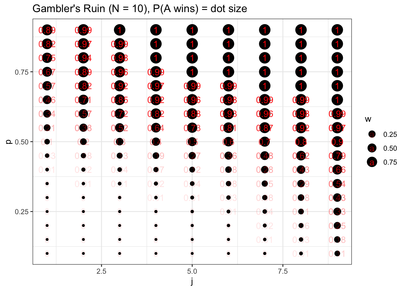
Here we vary \(j\) along the x-axis and \(p\) along the y-axis, and report the win probability of \(A\) with the size of the bubble (we also overlay text that reports the win probability with geom_text). It’s important to note here that \(p\) drives the win probability of \(A\) more than \(j\). We can see this visually: the dots change more when we move up and down than they do when we move left and right. Further, the edge cases are telling: when \(A\) only starts with \(j = 1\) dollars but has \(p = .9\) probability of winning each round, \(A\) has a \(.89\) probability of winning the entire game (the visual intuition here is that \(A\) has a \(.9\) probability of winning the game and going to \(j = 2, \; p = .9\) on the graph, which has a \(.99\) win probability). That is, even though \(A\) is starting with 1 dollar and \(B\) is starting with the rest (9 dollars), \(A\) is still the overwhelming favorite. Symmetrically, of course, this means that if \(A\) starts with 9 dollars but has \(p = .1\), he only has a \(.11\) probability of winning the game.
4.3.2 Expected Game Length
Another relevant question is a question of length: how long will these games last? Let’s consider a set-up as before: \(N\) dollars in the game, \(A\) starts with \(j\) dollars and has probability \(p\) of winning each round. Define \(M_j\) as the expected duration of the game if \(A\) starts with \(j\) dollars. We can write:
\[M_j = p(1 + M_{j + 1}) + q(1 + M_{j - 1})\]
Again by first-step conditioning (we have probability \(p\) of moving to \(j + 1\) dollars for \(A\) - and thus having expectation \(M_{j + 1}\) - and probability \(q\) of moving to \(j - 1\) - and thus we move to expectation \(M_{j - 1}\) - dollars for \(A\); we also add \(1\) because of that first step that we took).
We have simple edge cases: \(M_0 = M_N = 0\), since the game is over if \(A\) has \(0\) dollars or \(N\) dollars, by definition.
Anyways, let’s expand this equation:
\[M_j = p(1 + M_{j + 1}) + q(1 + M_{j - 1})\]
\[M_j = p + pM_{j + 1} + q + q M_{j - 1}\]
\[0 = pM_{j + 1} - M_j + q M_{j - 1} + 1\]
This is a non-homogeneous second order difference equation; again, we’re not going to delve deep into the proof behind the math here, so the approach may be a little hand-wavy.
We already saw that, for an equation of the form:
\[0 = pM_{j + 1} - M_j + q M_{j - 1}\]
A solution is:
\[M_j = c_1 + (\frac{q}{p})^jc_2\]
For a non-homogeneous difference equation, we take this result and add it to a particular solution of:
\[0 = pM_{j + 1} - M_j + q M_{j - 1} + 1\]
One solution that works is \(M_j = \frac{j}{q - p}\). We can plug this in:
\[0 = \frac{p(j + 1)}{q - p} - \frac{j}{q - p} + \frac{q(j - 1)}{q - p} + 1\]
Multiplying both sides by \((q - p)\), we get:
\[0 = pj + p - j + qj - q + q - p\]
\[= pj - j + qj\]
\[= j - j\] \[= 0\]
Excellent! So, \(\frac{j}{q - p}\) is a particular solution here. Adding to this to our general solution from earlier, we get:
\[M_j = c_1 + (\frac{q}{p})^jc_2 + \frac{j}{q - p}\]
Using the boundary condition \(M_0 = 0\), we get:
\[0 = c_1 + c_2\]
\[c_1 = -c_2\]
And the second boundary condition \(M_N = 0\), we get:
\[0 = c_1 + c_2(\frac{q}{p})^N + \frac{N}{q - p}\]
Plugging in \(c_2 = -c_1\):
\[0 = c_1 - c_1(\frac{q}{p})^N + \frac{N}{q - p}\]
\[-\frac{N}{q - p} = c_1(1 - (\frac{q}{p})^N)\]
\[c_1 = \frac{-\frac{N}{q - p}}{1 - (\frac{q}{p})^N}\]
And therefore:
\[c_2 = \frac{\frac{N}{q - p}}{1 - (\frac{q}{p})^N}\]
Plugging in for:
\[M_j = c_1 + (\frac{q}{p})^jc_2 + \frac{j}{q - p}\]
\[M_j = \frac{-\frac{N}{q - p}}{1 - (\frac{q}{p})^N} + (\frac{q}{p})^j \big(\frac{\frac{N}{q - p}}{1 - (\frac{q}{p})^N}\big) + \frac{j}{q - p}\]
Excellent! Unfortunately, there’s not a lot of algebra we can do to reduce this. We can write it in a more elegant way by splitting out the constants:
\[c_2 = \frac{N}{(q - p)\big(1 - (\frac{q}{p})^N)}\] \[c_1 = -c_2\]
\[M_j = c_1 + c_2 (\frac{q}{p})^2 + \frac{j}{q - p}\]
Where, remember, \(M_j\) is the expected length of a Gambler’s Ruin game with \(N\) total dollars where \(A\) starts with \(j\) dollars and has probability \(p\) of winning each round.
Note that, again, this is undefined for \(p = q\) (each of the terms would be dividing by \(0\)). We can go back to our original relation:
\[0 = pM_{j + 1} - M_j + q M_{j - 1} + 1\]
And remember from our solution of the win probability that a solution for an equation of the form \(0 = pM_{j + 1} - M_j + q M_{j - 1}\) where \(p = q\) is:
\[M_j = c_1 + c_2 j\]
We now need a particular solution to \(0 = pM_{j + 1} - M_j + q M_{j - 1} + 1\). We can try \(-j^2 = M_j\):
\[0 = -p(j + 1)^2 + j^2 + -q(j - 1)^2 + 1\] \[0 = -pj^2 - 2pj - p + j^2 - qj^2 + 2qj - q + 1\] \[0 = -j^2- p + j^2 - q + 1\] \[0 = -j^2 + j^2 - 1 + 1\] \[0 = 0\]
Excellent! It looks like \(-j^2\) is a particular solution, which means, continuing as we did in the \(p \neq q\) case, we have:
\[M_j = c_1 + c_2 j - j^2\]
Let’s now use our boundary conditions \(M_0 = 0\) and \(M_N = 0\). First, we have:
\[M_0 = 0 = c_1\]
And second, we have:
\[M_N = 0 = c_1 + Nc_2 - N^2\]
Plugging in \(c_1 = 0\) and rearranging, we have:
\[c_2 = N\]
Plugging in \(c_1\) and \(c_2\) in our equation for \(M_j\), we have:
\[M_j = Nj - j^2 = j(N - j)\]
This is the expected length of a game when \(p = q = 1/2\). We can quickly see for what value of \(j\) this is maximized by deriving w.r.t. \(j\), setting equal to zero and solving for \(j\):
\[M_j^{\prime} = N - 2j = 0\] \[j = \frac{N}{2}\]
This is intuitive; if the game is equally balanced, then the game will be longest if \(j\) is half of \(N\) (if both players have an equal chance of winning each round, then we expect the game to be longest if both players have an equal amount of money!).
We can code up this expectation and see how it changes as we vary the parameters:
FUN_ruinlength <- function(N, j, p) {

  # p = 1 / 2 case
  if (p == 1 / 2) {
    return(j * (N - j))
  }

  # other case
  q <- 1 - p
  c_2 <- N / ((q - p) * (1 - (q / p) ^ N))
  c_1 <- -c_2
  return(c_1 + c_2 * (q / p) ^ j + j / (q - p))
}


# initiate parameters and generate probabilities
N <- 10
j <- seq(from = 1, to = 9, by = 1)
p <- seq(from = .1, to = .9, by = .05)
mat <- expand.grid(j, p)
w <- apply(mat, 1, function(x) FUN_ruinlength(N, x[1], x[2]))

# visualize
data <- data.table(j = mat[ , 1], p = mat[ , 2], w = w)
ggplot() +
  geom_point(data = data, aes(x = j, y = p, size = w)) +
  theme_bw() +
  ggtitle("Gambler's Ruin (N = 10), E(Game Length) = dot size") +
  xlab("j") + ylab("p")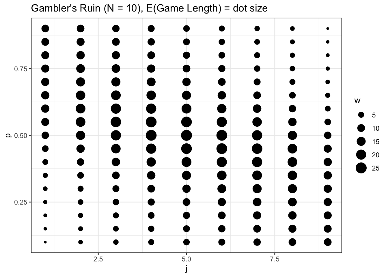
Intuitively, the closer that we get to a ‘fair game’ (\(j = 5\), which means that the players split the total amount of money \(N = 10\), and \(p = 1/2\), which means that each player has an equal probability of winning each round), the longer the games are expected to last. This time, interestingly, it seems that \(p\) and \(j\) both affect the expected game length a similar amount; unlike the previous win probability chart, the size of the dots don’t change more drastically when we look up and down vs. when we look left and right.
Finally, we can test that our solution actually makes sense by playing many Gambler’s Ruin games with some initial parameters and checking that the average game length is close to our analytically result. We can simulate this easily with the FUN_ruin function defined earlier in this chapter:
# replicate
set.seed(0)

# initialize parameters and generate results
p <- 1 / 3
j <- 5
N <- 10
results <- replicate(FUN_ruin(N = N, p = p, j = j), n = 1000)
results <- unlist(lapply(results, function(x) length(x) - 1))


# should match
mean(results); FUN_ruinlength(N, j, p)
## [1] 13.818## [1] 14.09091