Chapter 5 Branching Processes

“Make like a tree and get outta here.” -Biff

Motivation

We’ll now turn to yet another popular brand of stochastic processes, used frequently to model all sorts of real world phenomena (population growth, disease spread, etc.). These seemingly simply processes can quickly expand into nuanced complexities and pursuing their underlying structures, while sometimes challenging, is ultimately rewarding.

5.1 Simple Branching Processes

These processes are aptly named: they model the ‘branching out’ of some sort of population (for our purposes, let’s think of cells). Each cell lives for one time point and, at the end of the time point, either reproduces by creating some number of identical offspring (identical to the original cell) or doesn’t reproduce at all (and simply dies). This process continues independently with each of the remaining cells; if all the cells die out without reproducing, nothing else happens (the cells have gone extinct!).

We can formalize this with some notation. Let \(X_t\) count the number of living cells in generation \(t\). We define \(X_0 = 1\), which is essentially saying that there is one cell to start. The cell then has some ‘generation distribution’ which we will refer to as the offspring distribution:

\[\{p_0, p_1, p_2, ...\}\]

Where \(p_i\) is the probability that the cell has exactly \(i\) offspring. Note that \(\sum_{i = 0}^{\infty}p_i = 1\), so that we have a valid mass function.

Every cell that is created after the original cell has this identical generation distribution; also, the reproductions of every cell is independent of other cells. The population goes extinct as soon as, well, the population is of size zero! The extinction probability, which we will call \(p_e\), of the process is the probability that the process ever goes extinct.

Note that branching process are Markov; if we know how many cells are alive at time \(t - 1\) (which is \(X_{t - 1}\)), then no extra information from the history of the process matters in determining the distribution of \(X_t\). This is intuitive; we only care how many cells are alive in the period before (and thus how many will create reproductions), we don’t care how we got to that point!

Let’s start with some simple examples of branching processes.

1. \(p_0 = 1\) (and \(p_i = 0\) for \(i \geq 1\)). This is the most boring case: the original cell dies out and doesn’t reproduce at all (because the probability of producing zero offspring is one). The population is already extinct by \(t = 1\).

2. \(p_0 = 1/100\) and \(p_1 = 99/100\) (and \(p_i = 0\) for \(i \geq 2\)). Here, the cell either produces a single copy (with probability \(.99\)) or doesn’t reproduce at all (with probability \(.01\)). While the population might get lucky and survive for a while (and, indeed, over any one period, a living population will probability survive to the next period), the probability of surviving, say, to generation \(n\) is \(\frac{99}{100 ^ n}\) (since the population would need to reproduce successfully, with probability \(1/99\), for \(n\) generations). This goes to \(0\) as \(n\) gets large, so the probability of extinction for this population is \(1\).

We can simulate multiple paths of this process using a \(Geom(1/100)\) random variable (this counts the number of failures until a success in independent trials, where a success has probability \(1/100\) in every trial; of course, in this case, the ‘failures’ are the cell reproducing and the ‘success’ is the cell not reproducing). Even though we get some large values (\(843\) is our max here), all of the paths fail eventually (of course, simulating 10,000 paths isn’t a proof that this population will go extinct, it just helps with our intuition).

set.seed(0)
x <- rgeom(10000, .01)
max(x)

## [1] 843

3. \(p_0 = 1/4\), \(p_1 = 1/2\) and \(p_2 = 1/4\) (and \(p_i = 0\) for \(i \geq 3\)). This is our most complicated process so far: either the cell reproduces a single copy with probability \(1/2\), dies out without producing a copy with probability \(1/4\) or creates two copies with probability \(1/4\).

It is less clear how this population will fare in the long run. We can try simulating 500 different paths for 50 periods. Most of the paths collapse to zero (extinction), but plenty of populations are alive and well after 50 periods; one has more than 40 members!

set.seed(0)
nsims <- 500
index <- 50

# function to generate paths
FUN_branch <- function(index) {
  population <- 1
  for (i in 2:index) {
    population <- c(population, sum(sample(0:2, 
                                    population[length(population)],
                                    replace = TRUE,
                                    prob = c(1 / 4, 1 / 2, 1 / 4))))
  }
  population
}


# generate data and visualize
data <- data.table(t = 1:index, 
                   replicate(FUN_branch(index), n = nsims))
data <- melt(data, id.vars = "t")
ggplot(data, aes(x = t, y = value, col = variable)) +
  geom_line(alpha = 1 / 4) +
  theme_bw() +
  theme(legend.position = "none") +
  ggtitle("Simple Branching Process") +
  xlab("t") + ylab("size of population")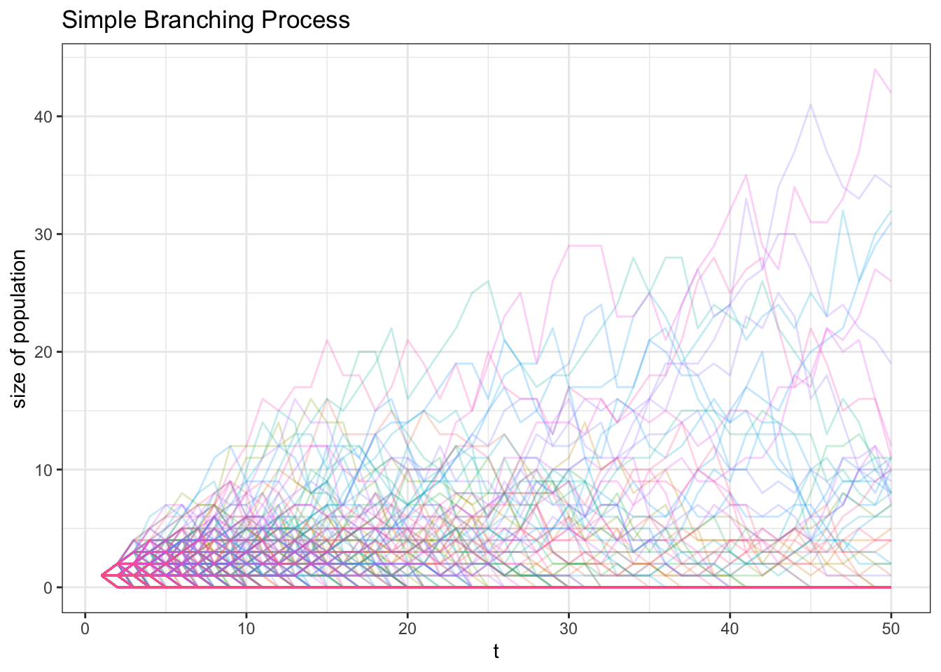

Here’s a video overview of this type of stochastic process:

Click here to watch this video in your browser

We’re going to develop a better framework for calculating the extinction probability of these processes. However, to do that, we need to learn about a new statistical tool.

5.2 Probability Generating Functions

The name already seems familiar, thanks to our work with Moment Generating Functions. We define the Probability Generating Function, or PGF, in a similar way. For a discrete random variable \(X\) with support \(0,1,2,...\), we have the PGF as:

\[\Pi_X(s) = E(s^X)\]

We use \(\Pi\) instead of \(P\) because, well, we already use \(P\) for probabilities! Also note that we have a notekeeping variable \(s\), similar to the \(t\) in the MGF.

Similar to the MGF, we can expand this using LOTUS:

\[\Pi_X(s) = E(s^X) = \sum_{x = 0}^{\infty} P(X = x)s^x\]

\[ = P(X = 0)s^0 + P(X = 1)s^1 + P(X = 2)s^2 + ...\]

The expansion in the last line is where we get part of the name of the PGF from; specifically, the coefficient on \(s^n\) is just \(P(X = n)\) (since each term in this expansion is \(P(X = n)s^n\) for \(n = 0, 1, 2....\)). This is the ‘Probability’ part in Probability Generating Function; we can generate these probabilities that \(X\) takes on different values quite easily by using the PGF.

First, if we just plug in \(0\) to our PGF, we can easily get the probability that \(X\) takes on \(0\).

\[\Pi_X(0) = \sum_{x = 0}^{\infty} P(X = x)0^x\] \[= P(X = 0) 0^0 + P(X = 1) 0^1 + P(X = 2) 0^2 + ...\] \[ = P(X = 0)\]

Since all of the \(0^x\) terms are \(0\) except for \(0^0\), which is \(1\). Therefore, we have that, as discussed:

\[\Pi_X(0) = P(X = 0)\]

This can also be a nice check to make sure that we have a valid PGF; plug in \(0\), and you should get \(P(X = 0)\).

How about generating the probability that \(X\) takes on the value \(1\)? Returning to our expansion of the PGF…

\[\Pi_X(s) = P(X = 0)s^0 + P(X = 1)s^1 + P(X = 2)s^2 + ...\]

…and taking the first derivative w.r.t. \(s\), we have:

\[\Pi_X^{\prime}(s) = P(X = 1) + 2s \cdot P(X = 2) + 3s ^ 2 \cdot P(X = 3) + ...\]

If we plug in \(0\) for \(s\), we are left with:

\[\Pi_X^{\prime}(0) = P(X = 1)\]

Continuing with this pattern, if we take another derivative of our PGF expansion, we get:

\[\Pi_X(s)^{\prime \prime} = 2P(X = 2) + 6s \cdot P(X = 3) + ...\]

Plugging in \(0\) for \(s\) here, we get:

\[\Pi_X(0)^{\prime \prime} = 2P(X = 2)\]

So we have:

\[\frac{\Pi_X(0)^{\prime \prime}}{2} = P(X = 2)\]

In general (deriving further), we see that:

\[\frac{\Pi_X(0)^{(n)}}{n!} = P(X = n)\]

Where the \((n)\) in the superscript simply means \(n^{th}\) derivative.

Fantastic! We have an easy way to calculate the probabilities of a random variable using its PGF (and now understand its name!). One final useful property comes into play when we plug \(1\) into our PGF:

\[\Pi_X(1) = P(X = 0)1^0 + P(X = 1)1^1 + P(X = 2)1^2 + ...\] \[ P(X = 0) + P(X = 1) + P(X = 2) + ...\] \[= 1\]

Because all of the \(s\) terms simply become \(1\). Thus, we have that \(\Pi_X(1) = 1\) (if you plug in \(1\) for \(s\) and don’t get \(1\) back, it’s not a valid PGF!).

Now that we are familiar with some properties, let’s actually try to calculate a PGF to introduce some concreteness. The simplest example is finding the PGF of \(X \sim Bern(p)\). Using the LOTUS expansion above:

\[\Pi_X(s) = E(s^X) = P(X = 0)s^0 + P(X = 1)s^1\] \[= (1 - p) + p \cdot s\]

That was easy! Let’s check that our two conditions, \(\Pi_X(0) = P(X = 0)\) and \(\Pi_X(1) = 1\), are satisfied.

\[\Pi_X(0) = (1 - p) + p \cdot 0 = (1 - p) = P(X = 0)\] \[\Pi_X(1) = (1 - p) + p = 1\]

The conditions check out! See below for a video introduction to these functions:

Click here to watch this video in your browser

Let’s now try to calculate the PGF of a slightly more complicated distribution: \(X \sim Bin(n, p)\). We could do the expansion above and perform a brute force calculation, or we could take this opportunity to learn about another useful property of PGFs.

Let \(Y\) and \(Z\) be independent random variables. Now let \(W = Y + Z\). What is the PGF of \(W\)?

We’ve seen this with MGFs; let’s start by writing out the PGF of \(W\) and plugging in \(Z + Y\):

\[\Pi_W(s) = E(s^W) = E(s^{Z + Y}) = E(s^Z s^Y)\]

Now, because \(Y\) and \(Z\) are independent, we can write:

\[E(s^Z s^Y) = E(s^Z)E(s^Y)\]

If you’re confused about this part, remember that we can expand \(E(s^Z s^Y)\) using two-dimensional LOTUS:

\[E(s^Z s^Y) = \sum_{z = 0} \sum_{y = 0} s^z s^y f(z, y)\]

Where \(f(z, y)\) is the joint mass function of \(Z\) and \(Y\). Since \(Z\) and \(Y\) are independent, the joint mass function is a product of the individual mass functions: \(f(z, y) = f(z) f(y)\). We can plug in and factor out:

\[= \sum_{z = 0} \sum_{y = 0} s^z s^y f(z) f(y)\] \[= \big(\sum_{z = 0} s^z f(z)\big) \cdot \big(\sum_{y = 0} s^y f(y)\big)\] \[=E(s^Z)E(s^Y)\]

Anyways, we are left with \(E(s^Z s^Y) = E(s^Z)E(s^Y)\), which essentially says the PGF of the sum of independent random variable is the product of the individual PGFs. This is something we can use for \(X \sim Binom(n, p)\), which is just a sum of \(n\) i.i.d. \(Bern(p)\), something we already have the PGF for! We thus have:

\[\Pi_X(s) = (1 - p + p \cdot s)^n\]

Checking our conditions:

\[\Pi_X(0) = (1 - p) ^ n = P(X = 0)\] \[\Pi_X(1) = (1 - p + p) ^ n = 1 ^ n = 1\]

It checks out!

Let’s turn to how the PGF can actually generate things other than probabilities. Similarly to the MGF, we will make use of derivatives. Specifically, we can calculate the first derivative w.r.t. \(s\):

\[\Pi_X(s)^{\prime} = E(X \cdot s^{X - 1})\]

If we plug \(1\) for \(s\), we get something familiar:

\[\Pi_X(1)^{\prime} = E(X)\]

Not bad; so taking the first derivative of the PGF and plugging in \(1\) generates the expectation of the random variable!

Let’s try taking another derivative:

\[\Pi_X(s)^{\prime \prime} = E(X(X - 1) \cdot s^{X - 2})\]

If we plug \(1\) in for \(s\) in this function, we are left with:

\[\Pi_X(1)^{\prime \prime} = E(X^2 - X) = E(X^2) - E(X)\]

That is, the second moment minus the first moment! We thus have, combining these two results:

\[E(X^2) = \Pi_X(1)^{\prime \prime} + \Pi_X(1)^{\prime}\]

Finally, we can check out this type of example in video form:

Click here to watch this video in your browser

5.3 Extinction Probabilities

Now that we have a handle on the PGF, we can try to use it to solve our original question: what is the probability of extinction for our branching process?

Let’s start by finding the PGF of a random sum of random variables. As you might be able to guess, this will be useful for branching processes, where the total reproduction of any single generation is a random sum of random variables, (it’s a ‘random sum’ because it depends on how many members of that generation there are). Let \(X = Y_1 + Y_2 + ... + Y_N\), where the \(Y\) terms are i.i.d. random variables with support \(0, 1, 2...\) and \(N\) is a random variable with support \(0, 1, 2...\).

What is the PGF of \(X\)? Let’s begin with the definition:

\[\Pi_X(s) = E(s^X) = \sum_{x = 0}^{\infty} P(X = x)s^x\]

Is there anything that we wish we knew? Well, to start, it would be helpful to know \(N\), since then we would at least know how many \(Y\) terms go into \(X\). Let’s try, then, conditioning on \(N\) (being sure to sum over all values of \(N\)):

\[= \sum_{n = 0}^{\infty} \sum_{x = 0}^{\infty} P(X = x|N = n)P(N = n)s^x\]

Since \(P(N = n)\) has nothing to do with \(X\), we can factor that out of the first sum:

\[= \sum_{n = 0}^{\infty}P(N = n) \sum_{x = 0}^{\infty} P(X = x|N = n)s^x\]

Hold on a moment…that \(\sum_{x = 0}^{\infty} P(X = x|N = n)s^x\) term is just the PGF of \(X\), conditioning on \(N = n\). Further, because \(N = n\) is fixed (we are conditioning on it), \(X\) is just the sum of \(n\) total \(Y\) random variables. So, we are looking for the PGF of a random variable \(X\) that is the sum of independent random variables \(Y_1 + Y_2 + ... + Y_n\). As we have seen above, the PGF of \(X\) is just, then, the product of the PGFs of the \(Y\) terms. Since the \(Y\) terms have identical distributions (they are i.i.d.), all of their PGFs are the same, and we can thus just write:

\[= \sum_{n = 0}^{\infty}P(N = n) \Big(\Pi_Y(s)\Big)^n\]

Now - and here’s where it gets really funky - doesn’t this equation just look like the PGF of \(N\), except we have the term \(\Big(\Pi_Y(s)\Big)\) where \(s\) would usually be? That means, dear reader, that this comes out to:

\[\Pi_N\Big(\Pi_Y(s)\Big)\]

Incredible! The PGF of \(X\) is just the PGF of \(Y\) fed into the PGF of \(N\). Formally, repeating the prompt from above, if \(X = Y_1 + Y_2 + ... + Y_N\), where the \(Y\) terms are i.i.d. random variables with support \(0, 1, 2...\) and \(N\) is a random variable with support \(0, 1, 2...\), then we have:

\[\Pi_X(s) = \Pi_N\Big(\Pi_Y(s)\Big)\]

Let’s now see how this property can be useful with extinction probabilities for branching processes. Let’s define our branching process as follows:

\[X_t = Y_{1, t - 1} + Y_{2, t - 1} + ... + Y_{X_{t - 1}, t - 1}\]

Where \(X_t\) is the size of the population at time \(t\) and \(Y_{i, t - 1}\) gives the number of offspring produced by the \(i^{th}\) member of the population at time \(t - 1\) (naturally, the total sum of these offspring constitute the population at time \(t\)). There are \(X_{t-1}\) of these \(Y\) terms because, well, there are \(X_{t-1}\) cells in the population at time \(t - 1\)!

Since we have that \(X_{t}\) is the sum of a random number \(X_{t-1}\) of random variables, we have, using our result from above, that the PGF of \(X_{t}\) is given by:

\[\Pi_{X_t}(s) = \Pi_{X_{t-1}} \Big(\Pi_{X_0}(s)\Big)\]

We write \(\Pi_{X_0}(s)\) here, or the generating function of the first cell in the population, because that is the generating function of all of the \(Y\) terms; each \(Y\) term generates offspring independently and with the same distribution as the first cell!

From here, we have some interesting iterations. We can use the above formula to find the PGF of \(X_{t - 1}\) in the same fashion:

\[\Pi_{X_{t - 1}}(s) = \Pi_{X_{t - 2}} \Big(\Pi_{X_0}(s)\Big)\]

Which, if we plug in to our expression for \(\Pi_{X_t}(s)\) above, yields:

\[\Pi_{X_t}(s) = \Pi_{X_{t - 2}} \Big(\Pi_{X_0}(\Pi_{X_0}(s))\Big)\]

If we continue in this way, we will get:

\[\Pi_{X_t}(s) = \Pi_{X_0}\Big(\Pi_{X_0}(...\Pi_{X_0}(s)...)\Big)\]

Where there are \(t\) of the \(\Pi_{X_0}\) terms.

It’s certainly complicated up to this point; it might help to review the following video recap before pressing on:

Click here to watch this video in your browser

Excellent! We now have the PGF of the branching process \(X_t\). Let’s now turn towards using this information to find \(p_e\), or the probability that the population goes extinct (with the help of material from this source).

We will need two key facts to find \(p_e\):

1. Recall that \(\Pi_{X_n}(0) = P(X_n = 0)\) (from above; plugging \(0\) into the PGF of \(X\) gives \(P(X = 0)\)). We also know that:

\[p_e = \lim_{n \to \infty} P(X_n = 0)\]

Because the right hand side of this equation is essentially giving the probability of the process going to zero as \(n\) goes to \(\infty\) (lots of time passes!) which is equivalent to the extinction probability \(p_e\). Plugging in \(\Pi_{X_n}(0) = P(X_n = 0)\) we have:

\[p_e = \lim_{n \to \infty} \Pi_{X_n}(0)\]

2. Recall what we showed above:

\[\Pi_{X_n}(0) = \Pi_{X_0}\Big(\Pi_{X_0}(...\Pi_{X_0}(0)...)\Big)\]

This fact implies that:

\[\Pi_{X_{n + 1}}(0) = \Pi_{X_0}(\Pi_{X_n}(0))\]

That is, we just add another \(\Pi_{X_0}\) to go from \(\Pi_{X_n}(0)\) to \(\Pi_{X_{n + 1}}(0)\).

With these two facts, we can begin a ‘chain of equality’ that gets us to our solution:

\[p_e = \lim_{n \to \infty} \Pi_{X_n}(0)\]

This is thanks to fact (1.) above.

\[\lim_{n \to \infty} \Pi_{X_n}(0) = \lim_{n \to \infty} \Pi_{X_{n + 1}}(0)\]

We are letting \(n\) go to infinity, so adding \(1\) in the subscript doesn’t change anything here (\(n\) and \(n + 1\) look much the same in the limit as \(n\) goes to \(\infty\)).

\[\lim_{n \to \infty} \Pi_{X_{n + 1}}(0) = \lim_{n \to \infty} \Pi_{X_0}(\Pi_{X_n}(0))\]

This is using fact (2.).

\[\lim_{n \to \infty} \Pi_{X_0}(\Pi_{X_n}(0)) = \Pi_{X_0}(\lim_{n \to \infty} \Pi_{X_n}(0))\]

We can do this because \(\Pi_{X_0}\), in the processes we are working with, is a continuous function. Finally, plugging in the result from (1.), we have:

\[\Pi_{X_0}(\lim_{n \to \infty} \Pi_{X_n}(0)) = \Pi_{X_0}(p_e)\]

And thus, the two ends of our chain of equality are:

\[p_e = \Pi_{X_0}(p_e)\]

Wow! This might not seem like much, but it means that we can set \(p_e\) equal to the PGF of the offspring distribution, \(\Pi_{X_0}\), with \(p_e\) as the input, and solve for \(p_e\). That is, we have an easy way to find our extinction probability by using the PGF!

We’ll do some examples shortly to let the power of this result sink in, but first we need a bit more housekeeping. Specifically, we can assert that \(p_e\), which is a probability and thus is between \(0\) and \(1\), is the smallest solution between \(0\) and \(1\) to the equation:

\[w = \Pi_{X_0}(w)\]

That is, there is no other valid probability that is the solution to the above and is smaller than \(p_e\).

We can prove this with some clever math. Imagine some value \(k\) (a value between \(0\) and \(1\)) that was also a solution, so we had:

\[k = \Pi_{X_0}(k)\]

We know that, from our original definitions, \(\Pi_{X_0}\) is an increasing function, so we must have:

\[\Pi_{X_0}(0) \leq \Pi_{X_0}(k) = k\]

We know the first bit \(\Pi_{X_0}(0) \leq \Pi_{X_0}(k)\) because \(0 \leq k\) by definition and thus plugging in \(k\) to \(\Pi_{X_0}\) will yield a value greater than or equal to the result from plugging in \(0\). We also know that \(\Pi_{X_0}(k) = k\) by definition; we said from the beginning that \(k = \Pi_{X_0}(k)\).

We can continue in this way, adding \(\Pi_{X_0}\) terms to both sides. The \(k\) doesn’t change, but we start to get:

\[\Pi_{X_0}\Big(\Pi_{X_0}(...\Pi_{X_0}(0)...)\Big) \leq k\]

Plugging in \(\Pi_{X_n}(0) = \Pi_{X_0}\Big(\Pi_{X_0}(...\Pi_{X_0}(0)...)\Big)\) from above, we get:

\[\Pi_{X_n}(0) \leq k\]

And letting \(n\) go to infinity, we get:

\[\lim_{n \to \infty} \Pi_{X_n}(0) \leq k\]

Of course, remember from fact (1.) above that we have \(\lim_{n \to \infty} \Pi_{X_n}(0) = p_e\), so we can just write:

\[p_e \leq k\]

Which proves that \(p_e\) is smaller than any other solution to:

\[w = \Pi_{X_0}(w)\]

This will be very useful if we find many solutions to this problem; just take the smallest one to get the correct probability of extinction!

Phew…that was a lot of math. Let’s do some examples of finding the extinction probability by using \(p_e = \Pi_{X_0}(p_e)\) to introduce some concreteness. Specifically, let’s go back to our process from before:

3. \(p_0 = 1/4\), \(p_1 = 1/2\) and \(p_2 = 1/4\) (and \(p_i = 0\) for \(i \geq 3\)).

Let’s calculate the PGF for this process:

\[E(s^X_0) = \Pi_{X_0}(s) = \sum_{x = 0}^{x = 2} P(X_0 = x)s^x\] \[=\frac{1}{4} + \frac{s}{2} + \frac{s ^ 2}{4}\]

We then use our result from earlier to solve for \(p_e\):

\[p_e = \Pi_{X_0}(p_e) = \frac{1}{4} + \frac{p_e}{2} + \frac{p_e ^ 2}{4}\]

Subtracting \(p_e\) from both sides, we get:

\[\frac{p_e ^ 2}{4} - \frac{p_e}{2} + \frac{1}{4} = 0\]

We can use R to code the quadratic equation and find the roots of the above:

FUN_quad <- function(a, b, c) {
  pos_root <- (-b + sqrt((b ^ 2) - 4 * a * c)) / (2 * a)
  neg_root <- (-b - sqrt((b ^ 2) - 4 * a * c)) / (2 * a)
  print(pos_root); print(neg_root)
}

FUN_quad(1 / 4, -1 / 2, 1 / 4)

## [1] 1
## [1] 1

We know that \(p_e\) is the smaller of these two solutions, and the solutions are the same, so \(p_e = 1\). That is, the population will go extinct with certainty! Let’s analyze a branching process with a more general structure.

4. You may have noticed that the offspring distribution of the process in the previous example was \(Bin(2, 1/2)\). Can we find a general solution for a process with offspring distribution \(Bin(2, p)\)? That is, what happens to the probability of extinction as \(p\), the probability of success (in each of the two independent trials for generating offspring), changes.

Recall that we found the PGF of a \(Bin(n, p)\) random variable earlier, so we can use that result here:

\[\Pi_{X_0}(s) = (1 - p + p \cdot s)^2\]

Using our result from earlier to find \(p_e\) and letting \(q = 1 - p\), we can write:

\[\Pi_{X_0}(p_e) = (q + p \cdot p_e)^2 = p_e\]

Let’s solve this out.

\[q^2 + p^2 p_e^2 + 2qpp_e = p_e\] \[p^2 p_e^2 + (2qp - 1)p_e + q^2 = 0\]

Plugging into the quadratic equation:

\[\frac{1 - 2qp \pm \sqrt{(1 - 2qp)^2 - 4q^2p^2}}{2p^2}\]

If we expand the \(\sqrt{(1 - 2qp)^2 - 4q^2p^2}}\), we get:

\[\sqrt{4q^2p^2 + 1 - 4qp - 4q^2p^2} = \sqrt{1 - 4qp}\]

Plugging back in:

\[=\frac{1 - 2qp \pm \sqrt{1 - 4qp}}{2p^2}\]

Let’s now plug in \((1 - p)\) for \(q\):

\[=\frac{1 - 2(1 - p)p \pm \sqrt{1 - 4(1 - p)p}}{2p ^ 2}\]

\[= \frac{1 - 2p + 2p^2 \pm \sqrt{1 - 4p + 4p^2}}{2p^2}\]

We can factor \(1 - 4p + 4p^2\) to get \((2p - 1)^2\), which means \(\sqrt{1 - 4p + 4p^2} = (2p - 1)\). Plugging in:

\[= \frac{1 - 2p + 2p^2 \pm (2p - 1)}{2p^2}\]

Let’s now split into the two cases. First, the \(+\) case:

\[\frac{1 - 2p + 2p^2 + (2p - 1)}{2p^2}\]

\[= \frac{2p^2}{2p^2} = 1\]

So, one of the solutions is \(1\). Let’s find the other solution with the \(-\) case:

\[\frac{1 - 2p - 2p^2 - (2p - 1)}{2p^2}\]

\[= \frac{2p^2 - 4p + 2}{2p^2}\]

Dividing by \(2\):

\[= \frac{p^2 - 2p + 1}{p^2}\]

Factoring \(p^2 - 2p + 1\) into \((p - 1)^2\), we get:

\[= \frac{(p - 1)^2}{p^2}\]

Of course, we know that \(p - 1 = -q\), so we get:

\[\frac{(-q)^2}{p^2} = \frac{q^2}{p^2}\]

Voila! Our two solutions are 1 and \(\frac{q^2}{p^2}\).

Remember that \(p_e\), the probability of extinction, is the minimum of our solutions. Therefore, we have that:

\[p_e = min(1, \frac{q^2}{p^2})\]

This certainly was a lot of algebra; the video below wors through the same derivation and might help to build understanding:

Click here to watch this video in your browser

Let’s see if we can get some intuition around this. If \(p\) is very large, then \(\frac{q^2}{p^2}\) get small, which means \(p_e\) gets small; this makes sense, because \(p\) is the probability of generating offspring (on each of the 2 independent trials) and thus a higher value of \(p\) means a lower extinction probability \(p_e\) (and vice versa for \(q\); when \(q\) is large, \(p_e\) is large). It also makes sense that \(p_e\) maxes out at \(1\); it’s a probability, it can’t go any higher than 1.

We can easily visualize this result in R. Unsurprisingly, a larger \(p\) reduces the probability of extinction; interestingly, if \(p \leq .5\), then we have \(p_e = 1\). That is, if \(p\) is \(.5\) or less, the population will go extinct; more on this in a moment.

p <- seq(from = .01, to = 1, by = .01)
data <- data.table(p = p,
                   p_e = (1 - p) ^ 2 / p ^ 2)
data$p_e[data$p_e > 1] <- 1

ggplot(data, aes(x = p, y = p_e)) +
  geom_point() +
  theme_bw() +
  xlab("p") + ylab("Extinction Probability") +
  ggtitle("Extinction Probability for Bin(2, p) offspring distribution")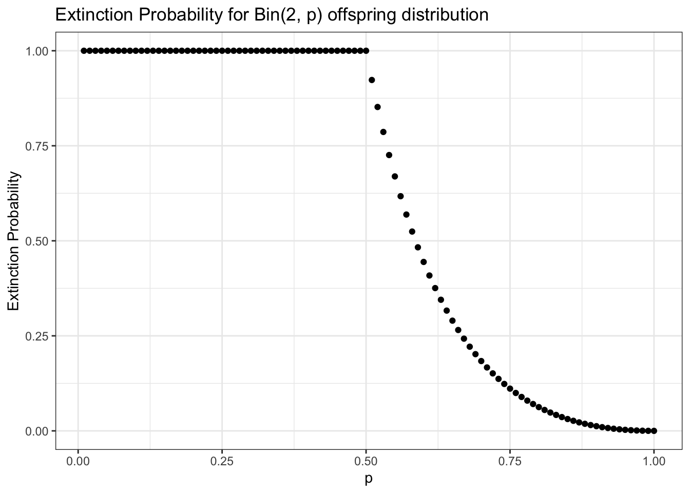

5.4 Extinction Conditions

We see in the above chart an interesting pattern; the probability of extinction for \(p\leq .5\) is simply 1 (i.e., the population will definitely go extinct). In fact, there is a simple, useful way to tell if a branching process will go extinct or might go extinct; we explore that here (with help from this resource).

Like we did above, let’s define \(\Pi_{X_0}(s)\) as the PGF of the ‘offspring distribution.’ Remember that we start with one individual cell at time \(t = 0\) and then this cell reproduces according to some distribution, which we call here \(X_0\) (i.e., so that \(E(X_0)\) is the expected value of the offspring distribution). Each new cell that is created reproduces independently according to this same distribution. We also showed in the earlier section that the smallest solution to \(w = \Pi_{X_0}(w)\) gives \(p_e\), or the extinction probability of the process.

Let’s talk about convexity. Remember that a convex function has a positive second derivative; the second derivative of \(x^2\) w.r.t. \(x\), for example, is \(2\).

data <- data.table(x = 0:100,
                   y = (0:100) ^ 2)
ggplot(data, aes(x = x, y = y)) +
  geom_line() +
  theme_bw() +
  xlab("x") + ylab("y = x ^ 2") + ggtitle("Convex Function")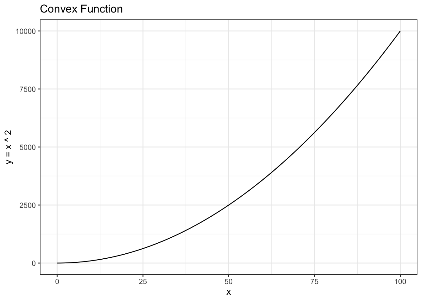

Similarly, a concave function has a negative second derivative. For example the second derivative of \(\sqrt{x}\) is \(\frac{-x^{\frac{-3}{2}}}{4}\).

data <- data.table(x = 0:100,
                   y = sqrt(0:100))
ggplot(data, aes(x = x, y = y)) +
  geom_line() +
  theme_bw() +
  xlab("x") + ylab("y = sqrt(x)") + ggtitle("Concave Function")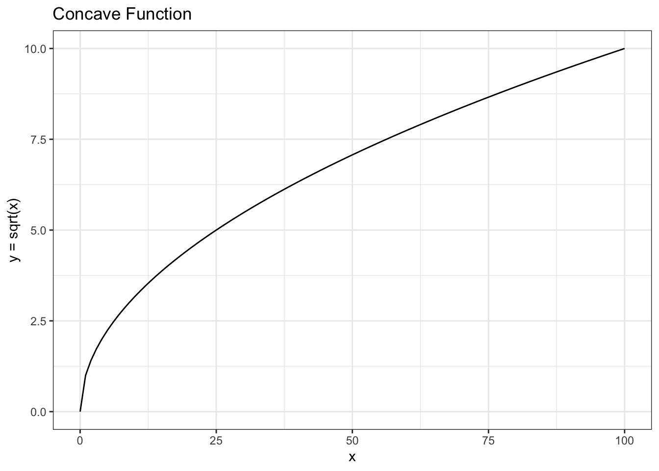

Is our PGF \(\Pi_{X_0}(s)\) convex or concave on the interval \(0 \leq s \leq 1\) (this interval is all that we will worry about, because we are looking for the extinction probability \(p_e\) that is the solution to \(p_e = \Pi_{X_0}(p_e)\), and \(p_e\) must be on the interval 0 to 1 because it is a probability)? Let’s write out our PGF again:

\[\Pi_{X_0}(s) = E(s^{X_0}) = \sum_{x = 0}^{\infty} s^xP(X = x)\] \[ = P(X = 0) + s P(X = 1) + s^2P(X = 2) + ...\]

As well as the derivative of our PGF:

\[\Pi_{X_0}^{\prime}(s) = P(X = 1) + 2sP(X = 2) + ...\]

Let’s only consider branching processes with \(P(X > 1) > 0\); that is, the offspring distribution can take on a value of 2 or more. Otherwise, we get pretty uninteresting processes: the cell either makes 1 copy or zero copies and, unless it makes 1 copy with probability 1 (which is also boring; just one cell in each generation for the rest of time!), will thus definitely die out eventually.

If \(P(X > 1) > 0\), then both \(\Pi_{X_0}(s)\) and \(\Pi_{X_0}^{\prime}(s)\) are strictly increasing functions in terms of \(s\), because all of the terms are non-negative (remember that \(s\) is between \(0\) and \(1\)) and at least one of the terms that varies with \(s\) (i.e., \(s^2 P(X = 2)\)) is not \(0\) (we can just look at the equations; it’s clear that they are increasing with \(s\)).

Since the first derivative \(\Pi_{X_0}^{\prime}(s)\) is strictly increasing on the interval, we have that the PGF is convex. We can thus make a useful chart:

This chart has a lot of important hidden complexities. Let’s walk through what is happening here.

• The blue line is the output of the PGF \(\Pi_{X_0}(s)\). For different values \(s\) on the horizontal axis, we see the output of \(\Pi_{X_0}(s)\) on the vertical axis (labeled here as \(y\)). As we have shown, this line is convex (which we can see here visually).
• The black line is simply the unit line with slope 1 (or \(y = s\)).
• Note that the location where the blue line \(\Pi_{X_0}(s)\) intersects the y-axis is \(P(X_0 = 0)\), or the probability of zero offspring according to the offspring distribution. This makes sense because remember one of the first properties that we saw of the PGF: \(\Pi_{X_0}(0) = P(X_0 = 0)\).
• The point where the blue line (the PGF) crosses the unit line is \(p_e\), the extinction probability. That’s because, remember, \(p_e\) is the smallest solution to \(w = \Pi_{X_0}(w)\), and the intersection of the blue line (the PGF) and the unit line (along which every point we have \(s = t\)) provides this value. Also not that this intersection is the smallest solution to \(w = \Pi_{X_0}(w)\), because the blue and black lines also intersect at \(s = 1\). This was also a key property of PGFs that we learned about earlier: \(\Pi_{X_0}(1) = 1\).
• Finally, remember that we showed how \(\Pi_{X_0}^{\prime}(1) = E(X_0)\). Therefore, the slope of the blue line (PGF) at \(s = 1\) is just \(E(X_0)\), or the mean of the offspring distribution!

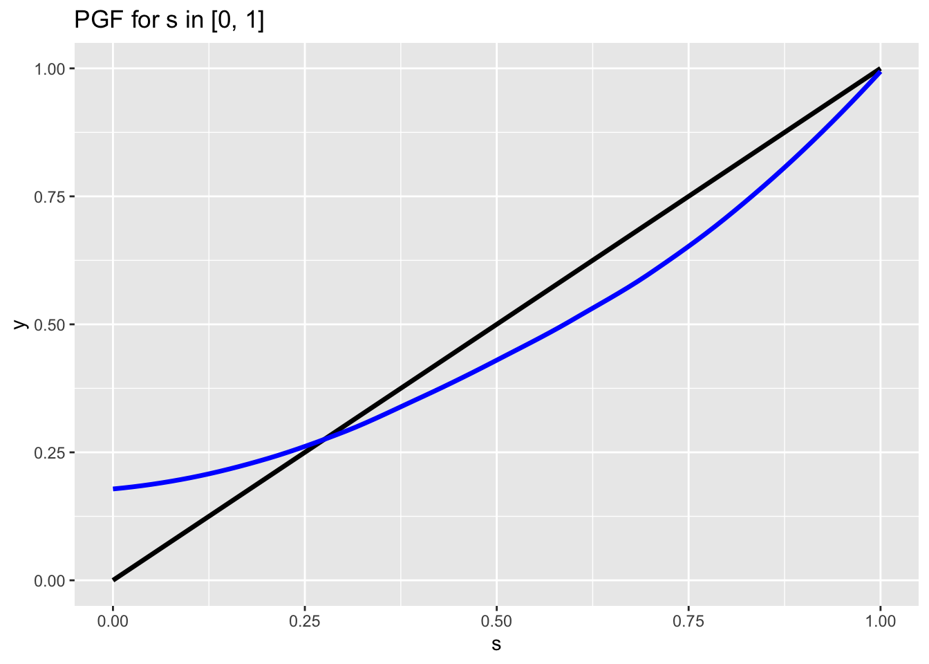
Now comes the really cool part. We’ve seen that \(E(X_0)\) defines the slope of the PGF at 1. Let’s consider the case where \(E(X_0) < 1\). Our chart could look something like this:

Note that, because \(E(X_0) < 1\), the blue line stays entirely above the black line until \(s = 1\). This is obviously the case in the above chart, but it’s also the case whenever \(E(X_0) < 1\). The reason is because, since the slope is less than 1, as we move backward from \(s = 1\) the blue line will not fall as quickly as the black line and thus the black line will be under the blue line. As we move closer to \(s = 0\), the slope will get even smaller (because we showed that the PGF is a convex function from \(s = 0\) to \(s = 1\) and thus the slope increases on this interval) and the blue line will never catch the black line before \(s = 0\).

What’s the implication here? Well, since we get \(p_e\), the probability of extinction, from the intersections of the blue and black line, and the only intersection possible is at \(s = 1\) (we showed above how they will not intersect again by \(s = 0\)), we can therefore say that \(p_e = 1\), or the population will definitely go extinct if the expected value of the offspring distribution is less than 1 (\(E(X_0) < 1\)).

In fact, the same holds if \(E(X_0) = 1\), since the slope of the blue line will be 1 at \(s = 1\) but strictly smaller for \(s < 1\) and thus won’t cross the black line either (the exception is when \(P(X_0) = 1\), or the offspring distribution is simply always 1 with no variance, in which case the PGF will just be the unit line; this is a pretty uninteresting case though, since this population will clearly not go extinct). Therefore, we can amend our statement above: the population will definitely go extinct if the expected value of the offspring distribution is less than or equal to 1 (\(E(X_0) < 1\)).

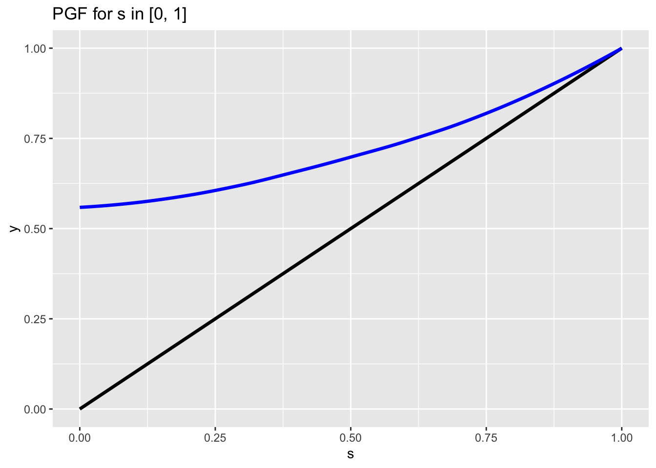
How about the final case? Our first chart gave a good example of when \(E(X_0) > 1\):

## `geom_smooth()` using method = 'loess' and formula 'y ~ x'

Here, the slope of the blue line (PGF) at \(s = 1\) is greater than 1, which, for symmetrical reasons to the ones discussed before (slope is larger than the black unit line, so it will fall faster and thus be below the black line), ensures that we will have the blue line intersect the black line again somewhere between \(s = 0\) and \(s = 1\) and thus have a solution \(p_e\) that is smaller than \(1\). Even the edge case works here: if we have \(P(X_0 = 0) = 0\), in which case the blue line just intersects the black line at \(s = 0\), this means that \(p_e = 0\), or the population will certainly not go extinct. This makes sense, because \(P(X_0 = 0) = 0\) means ‘there is a zero probability that a cell has zero offspring’ which just means that the cells would reproduce with certainty! Therefore, we can say the population will not certainly go extinct (it might go extinct, it’s just not a certainty) if the expected value of the offspring distribution is greater than 1 (\(E(X_0) > 1\)).

This is definitely a different sort of derivation, and perhaps better suited to video form:

Click here to watch this video in your browser

These are very powerful results; we can immediately say if a process will definitely go extinct by just looking at the offspring distribution. It makes sense intuitively: if, on average, each cell is producing less than one cell for the next generation, the population will not fare well!

5.5 Long-term Population Metrics

We’ve done most of the heavy lifting, so it’s time to think about some of the key measurements of branching process populations in the long term. First (with help from this resource), let’s think about what the mean of some branching process \(X_t\) is; that is, \(E(X_t)\) (or the expected size of the population at time \(t\)). Let’s use \(\mu_t\) for our notation here, and \(\mu\) as the mean of the offspring distribution (i.e., the average number of cells reproduced by each cells).

We can calculate \(\mu_t\) by using key facts of the PGF. Specifically, remember that:

\[\Pi_{X_t}^{\prime}(1) = \mu_t\]

That is, plugging \(1\) into the derivative of the PGF of \(X_t\) gives the mean of \(X_t\). Let’s start then, with the PGF of \(X_t\). Remember what we showed above:

\[\Pi_{X_t}(s) = \Pi_{X_{t - 1}}(\Pi_{X_0}(s))\]

Taking the derivative of both sides (remember to use the chain rule on the right side; the derivative of the function \(\Pi_{X_{t - 1}}\) and then the derivative of the input to that function \(\Pi_{X_0}(s)\)):

\[\Pi_{X_t}^{\prime}(s) = \Pi_{X_{t - 1}}^{\prime}(\Pi_{X_0}(s))\Pi_{X_0}^{\prime}(s)\]

Now let’s plug in \(1\) for \(s\):

\[\Pi_{X_t}^{\prime}(1) = \Pi_{X_{t - 1}}^{\prime}(\Pi_{X_0}(1))\Pi_{X_0}^{\prime}(1)\]

Using the fact that \(\Pi_{X_t}^{\prime}(1) = \mu_t\) and \(\Pi_{X_0}(1) = 1\), we have:

\[=\Pi_{X_{t - 1}}^{\prime}(1)\Pi_{X_0}^{\prime}(1)\] \[ =\Pi_{X_{t - 1}}^{\prime}(1) \mu\]

Where, remember, \(\mu\) is the mean of the offspring distribution. Therefore, we have:

\[\Pi_{X_t}^{\prime}(1) = \mu_t = \Pi_{X_{t - 1}}^{\prime}(1) \mu\]

We could continue in this way:

\[= \Pi_{X_{t - 2}}^{\prime}(1) \mu^2\]

Until we get to:

\[\mu_t = \mu^t\]

Excellent! We have arrived at the intuitive result that the average size of the population at time \(t\) is just the mean of the offspring distribution raised to the value \(t\) (it makes sense because each reproduced cell has the same offspring distribution, so there is a compounding effect).

We can also note that this meshes with our earlier extinction probability conditions. If \(\mu < 1\), which we’ve seen is a condition that means the population will go extinct with probability \(1\), we have that \(\mu^t\) approaches \(0\) as \(t\) goes to \(\infty\) (i.e., it goes extinct!). When \(\mu = 1\), of course, we have that \(\mu^t = 1\) for all \(t\) (remember that this population will also go extinct with certainty except in the degenerate case of \(P(X_0 = 1) = 1\), or the offspring distribution can only take on the value \(1\) with certainty).

If \(\mu > 1\), then clearly \(\mu^t\) gets large and approaches \(\infty\) as \(t\) goes to \(\infty\). Again, this meshes with the result we saw earlier: a population with \(\mu > 1\) will not definitely go extinct (although they will have some extinction probability).

We can use the above result \(E(X_t) = \mu^t\) to find the expected value of the total individuals in the history of the population until time \(t\) (i.e., all individuals who have ever lived up to time \(t\)). Let’s define this as \(M_t\). By definition, we have that:

\[M_t = X_0 + X_1 + X_2 + ... + X_t\]

Or the size of all of the generations up through time \(t\). Taking the expectation of both sides (and using linearity of expectation, and remembering that \(X_0 = 1\) by definition):

\[E(M_t) = E(X_0 + X_1 + X_2 + ... + X_t)\] \[E(M_t) = E(X_0) + E(X_1) + E(X_2) + ... + E(X_t)\] \[E(M_t) = 1 + \mu + \mu^2 + ... + \mu^t\]

Voila! This is relatively easy to calculate and allows us to think about the long-term total population size for different populations. If we have \(\mu > 1\), again, the series \(1 + \mu + \mu^2 + ... + \mu^t\) clearly goes to \(\infty\) as \(t\) goes to infinity (the expected total population size gets very large as time passes). If we have \(\mu = 1\), then \(E(M_t) = t\), which makes sense; if we expect just one cell to be reproduced each time, then, after \(t\) time, we expect \(t\) total cells! Finally, if \(\mu < 1\), we have that \(E(M_t)\) converges (it’s just a geometric series!) to:

\[=\frac{1}{1 - \mu}\]

Larger values of \(\mu\) will thus make the expected total population size larger; for example, if \(\mu = .99\), then \(E(M_t) = 100\), and if \(\mu = .01\), then \(E(M_t)\) is slightly larger than \(1\). This makes sense, because if the offspring distribution has a higher mean, we expect the total size of the population to be larger (note that in the \(\mu = .01\) case, the expected value of the population is just slightly above \(1\), because there is a good chance that the first cell doesn’t reproduce at all!).

Here is a video demonstration of this solution:

Click here to watch this video in your browser

Now that we’ve found \(E(X_t)\), let’s finally turn to finding the variance of \(X_t\). We will similarly denote this with \(\sigma^2_t\). Recall the derivative that we worked with on the last problem:

\[\Pi_{X_t}^{\prime}(s) = \Pi_{X_{t - 1}}^{\prime}(\Pi_{X_0}(s))\Pi_{X_0}^{\prime}(s)\]

Deriving again (remember the product rule; derivative of the first term times the second term, plus the derivative of the second term times the first term) we get:

\[\Pi_{X_t}^{\prime \prime}(s) = \Pi_{X_{t - 1}}^{\prime \prime}(\Pi_{X_0}(s))\big(\Pi_{X_0}^{\prime}(s)\big)^2 + \Pi_{X_{t - 1}}^{\prime}(\Pi_{X_0}(s))\Pi_{X_0}^{\prime \prime}(s)\]

Remember that \(\Pi_{X_0}^{\prime \prime}(1) = \sigma^2 - \mu + \mu^2\) from above (we had the property of the PGF that \(\Pi_{X}^{\prime \prime}(1) = E(X^2) - E(X)\), and we can re-write \(E(X^2)\) as \(Var(X) + E(X)^2\) so that we are left with \(\Pi_{X}^{\prime \prime}(1) = Var(X) + E(X)^2 - E(X)\)), so we have:

\[\Pi_{X_t}^{\prime \prime}(1) = \sigma^2_t - \mu^t + \mu^{2t}\] \[\Pi_{X_{t-1}}^{\prime \prime}(1) = \sigma^2_{t-1} - \mu^{t-1} + \mu^{2t - 2}\]

Since \(E(X_t) = \mu^t\) and \(E(X_{t - 1}) = \mu^{t - 1}\).

Combining this with the facts that we used earlier (\(\Pi_{X_0}(1) = 1\) and \(\Pi_{X_0}^{\prime}(1)\)), we can plug in \(1\) for \(s\) into our second derivative above:

\[\Pi_{X_t}^{\prime \prime}(1) = \Pi_{X_{t - 1}}^{\prime \prime}(\Pi_{X_0}(1))\big(\Pi_{X_0}^{\prime}(1)\big)^2 + \Pi_{X_{t - 1}}^{\prime}(\Pi_{X_0}(1))\Pi_{X_0}^{\prime \prime}(1)\]

Plugging in on both sides:

\[\sigma_t^2 - \mu^t + \mu^{2t} = (\sigma_{t - 1}^2 - \mu^{t - 1} + \mu^{2t - 2}) \cdot \mu^2 + \mu^{t - 1} \cdot(\sigma ^ 2 - \mu + \mu^2)\]

And now we can just solve for \(\sigma_t^2\):

\[\sigma_t^2 = \mu^t - \mu^{2t} + \sigma_{t - 1}^2 \cdot \mu^2 - \mu^{t - 1} \cdot \mu^2 + \mu^{2t - 2} \cdot \mu^2 + \sigma ^ 2 \cdot \mu^{t - 1} - \mu \cdot \mu^{t - 1} + \mu^2 \cdot \mu^{t - 1}\]

\[\sigma_t^2 = \mu^t - \mu^{2t} + \sigma_{t - 1}^2 \cdot \mu^2 - \mu{t + 1} + \mu^{2t} + \sigma ^ 2 \cdot \mu^{t - 1} - mu^t + \mu^{t + 1}\]

\[\sigma_t^2 = \sigma_{t - 1}^2 \cdot \mu^2 + \sigma ^ 2 \cdot \mu^{t - 1}\]

This means we also know \(\sigma_{t - 1}^2\) (we can just use the above equation):

\[\sigma_{t - 1}^2 = \sigma_{t - 2}^2 \cdot \mu^2 + \sigma ^ 2 \cdot \mu^{t - 2}\]

So we can plug this in to our equation for \(\sigma_t^2\) to get:

\[\sigma_t^2 = \mu^2\big(\sigma_{t - 2}^2 \cdot \mu^2 + \sigma ^ 2 \cdot \mu^{t - 2}\big) + \sigma ^ 2 \cdot \mu^{t - 1}\]

\[\sigma_t^2 = \sigma_{t - 2}^2 \mu^4 + \sigma^2 \cdot \mu^t + \sigma^2 \mu^{t - 1}\]

And now plugging in for \(\sigma_{t - 2}^2\) which, by the same pattern, is:

\[\sigma_{t - 1}^2 = \sigma_{t - 3}^2 \cdot \mu^2 + \sigma ^ 2 \cdot \mu^{t - 3}\]

\[\sigma_t^2 = \mu^4\big(\sigma_{t - 3}^2 \cdot \mu^2 + \sigma ^ 2 \cdot \mu^{t - 3}\big) + \sigma^2 \cdot \mu^t + \sigma^2 \mu^{t - 1}\]

\[\sigma_t^2 = \mu^6 \sigma_{t - 3}^2 + \sigma ^ 2 \cdot \mu^{t + 1} + \sigma^2 \cdot \mu^t + \sigma^2 \mu^{t - 1}\]

Note that the \(\sigma^2\) terms are growing; also note that the \(\mu^6 \sigma_{t - 3}^2\) term keeps adding \(2\) in the exponent each time that the increment of \(\sigma\) goes down by 1. Eventually, we will get \(t = 1\), where we have \(\sigma_1 = \sigma\), since this is just the variance of the offspring distribution (at \(t = 1\), we just have the offspring from the original cell in \(t = 0\)). Therefore, after taking \(t - 1\) steps down to time \(t = 1\), we have:

\[\sigma_t^2 = \mu^{2t - 2} \sigma + \sigma ^ 2 \cdot \mu^{2t - 3} + ... + \sigma ^ 2 \cdot \mu^{t + 1} + \sigma^2 \cdot \mu^t + \sigma^2 \mu^{t - 1}\]

Factoring out \(\mu^{t - 1}\), we have:

\[\sigma_t^2 = \mu^{t - 1}\sigma^2(1 + \mu + \mu^2 + ... + \mu^{t - 1})\]

Excellent! We can immediately see that if \(\mu = 1\), we are just left with:

\[\sigma_t^2 = t \cdot \sigma^2\]

Which makes sense (the variance increases with time \(t\)). We can also see that if \(\mu > 1\), this sum will go to \(\infty\) as \(n\) goes to \(\infty\), and if \(\mu < 1\), it will converge (using the geometric series) to:

\[\frac{\mu^{t - 1} \sigma^2}{1 - \mu}\]