Chapter 1 Introduction
1.1 What is Statistics?
Video 1: What is Statistics?
Statistics is the field of mathematics concerned with reasoning about data and uncertainty.
This includes collecting, organising, summarising, analysing and presenting data.
In particular, Statistics provides the tools for making decisions and drawing conclusions from data in a principled way—this is called statistical inference.
A key part of statistics is communicating: communicating context, data, assumptions, analysis, results.
1.2 Populations and samples
A key idea in Statistics is to draw conclusions about a population based on a sample from that population. This is where the word inference comes from: we are inferring something about the population based on the sample.
Population
A population is a group or collection of similar individuals (e.g. students), items (e.g. plants) or events (e.g. days) that are of interest to us.
When we want to make inferences about a population, it would be very time consuming and expensive to look at every member of the population. It could also be destructive if the experiment involves testing until failure.
Sample
A sample is a subset of the population.
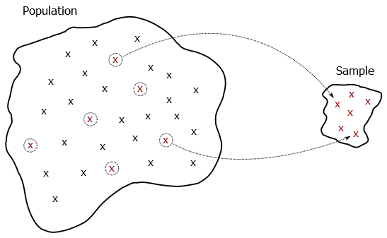
Figure 1.1: A sample is a subset of the population. Each x here represents a sampling unit; red shows the ones in the sample.
Population: The students studying mathematics.
Sample A: Those students who were born in London.
Sample B: Female students.
Population: Female students at University of Nottingham.
Sample A: Ten randomly chosen female students.
Sample B: Ten randomly chosen female students from mathematics.
If inferences about the population based on sample data are to make sense, the sample must be representative of the population.
In Example 1, neither Sample A nor Sample B are very representative of the population. Suppose, say, we wanted to infer the proportion of all students on this module that are over 1.8m tall: why would basing the inference on a sample of only females be a bad idea?
In Example 2, these samples are random samples. Random sampling is often used to help ensure the sample is representative of population.
The individual items in the population and sample are called elements or sampling units. In conducting an experiment we are trying to learn about particular aspects or phenomena of the population of elements. These unknown phenomena are known as random variables and in an experiment we observe a random variable on each element in the sample in order to make inferences about the values of the random variable in the population.
Often the population is large enough compared to the sample size to be assumed infinite; e.g., the population of the UK is much greater than a sample of 100 taken from that population.
Population: Everyone in the UK.
Random variable: Height.
Take a random sample of people and measure their height.
Population: Litters of one breed of dog.
Random variable: Number of puppies in a litter.
Take a random sample of litters and count the number of puppies in each
litter.
1.3 Types of Data
A measurement of a random variable is commonly termed an observation and a collection of observations is called data. The set of outcomes that an observation can take is called the sample space and we formalise this in Section 4.3 when we introduce probability.
There are many different types of data. There are two main types of data, numerical (quantitative) and categorical (qualitative) data:
Numerical data
Discrete
Numerical values taking a discrete (usually integer) set of values. (Finite or infinite number of possibilities.)
Example: How many siblings do you have?
Continuous
Numerical values taking values on a continuous range. (Finite or infinite range.)
Example: What is your height in cm?
and
Categorical data
Nominal
Set of values that don’t possess a natural ordering.
Example: What is your eye colour?
Ordinal
Set of values that do possess a natural ordering.
Example: Letter grades for assessment.
Binary
Only two possible outcomes.
Example: Do you have a brother?
Enter your data into the Microsoft form. This data will be used anonymously (with data from another course) at various stages in the module. Think about the type of data generated for each question.
Data: Microsoft Form
1.4 Some example datasets
Three data sets we’ll use in the Section 2 are as follows.
Cavendish experiment
In 1798, Henry Cavendish conducted an experiment
to estimate the density of the earth. His 29 measurements, presented as
a multiple of the density of water were:
| 5.50 | 5.57 | 5.42 | 5.61 | 5.53 | 5.47 | 3.88 | 5.62 | 5.63 | 5.07 |
| 5.29 | 5.34 | 5.26 | 5.44 | 5.46 | 5.55 | 5.34 | 5.30 | 5.36 | 5.79 |
| 5.75 | 5.29 | 5.10 | 5.86 | 5.58 | 5.27 | 5.85 | 5.65 | 5.39 |
Coursework marks
The marks of 18 students on a piece of coursework
are:
| Mark | 34 | 42 | 44 | 46 | 48 | 50 |
|---|---|---|---|---|---|---|
| Frequency | 1 | 2 | 3 | 6 | 3 | 3 |
Optometry data
Optometry measurements of eye pressure (IOP/\(mmHg\)) taken by 40 students. 20 Optometry students and 20 engineering students.
Optometry students
| 14 | 15 | 15 | 14 | 15 | 15 | 15 | 14 |
| 15 | 16 | 15 | 15 | 16 | 15 | 15 | 15 |
| 15 | 16 | 15 | 15 |
Engineering students
| 16 | 15 | 17 | 19 | 15 | 17 | 13 | 13 |
| 13 | 23 | 10 | 13 | 20 | 18 | 16 | 12 |
| 10 | 17 | 8 | 15 |
1.5 Statistical Computing
Throughout this module, and indeed the MSc programme, we will be supporting the statistical theory and methodology with applications using the statistical package R. Whilst it is important to understand the theory behinds statistical methods it is very rare to implement statistical methods by hand and R or another statistical package is used. The old computing adage GIGO (garbage in, garbage out) is relevant to statistical computing. If we will tell R to do something such as perform a calculation, fit a model or predict future observations, it probably will, but we need to be able to check that the question asked, and the answer given, make sense.
1.6 The statistical paradigm
We have introduced data types and the concept of obtaining a sample from a population. We are now in position to outline the steps involved in statistical analysis from identification of population and research question of interest through the statistical analysis to interpretation and communication of the analysis.
Statistical analysis consists of a number of steps:
- Specification of population
- Identification of research question
- Sampling design of a protocol
- Data collection
- Exploratory analysis
- Model specification
- Diagnostics (Model verification)
- Inference
- Interpretation
- Communication
The procedure is not usually linear - some iteration may be necessary.
In the following Sections we discuss ways to summarise (Section 2) and visualise (Section 3) our data before we introduce probability (Section 4) which underpins the mathematical modelling and analysis of data.
Task: Lab 1
In Section 23, an introduction to the statistical package R is given. This includes downloading R and getting started.
Work through Section 23 and then attempt:
Lab 1: Introduction to R