Chapter 10 Techniques for Deriving Estimators

10.1 Introduction

In this Section we introduce two techniques for deriving estimators:

• Method of Moments
  
• Maximum Likelihood Estimation

The Method of Moments is a simple, intuitive approach, which has its limitations beyond simple random sampling (i.i.d. observations). Maximum Likelihood Estimation is an approach which can be extended to complex modelling scenarios and likelihood based estimation procedures will be central to statistical inference procedures throughout not only this module but the whole course.

10.2 Method of Moments

Let \(X\) be a random variable.

If \(E[X^k]\) exists in the sense that it is finite, then \(E[X^k]\) is said to be the \(k^{th}\) moment of the random variable \(X\).

For example,

• \(E[X] = \mu\) is the first moment of \(X\);

• \(E[X^2]\) is the second moment of \(X\).

Note that \(var(X) = E[X^2] - (E[X])^2\) is a function of the first and second moments.

Let \(X_1, X_2, \ldots, X_n\) be a random sample. The \(k^{th}\) sample moment is

\[\hat{\mu}_k = \frac{1}{n} \sum_{i=1}^n X_i^k.\]

Since, \[\begin{align*} E[\hat{\mu}_k] &= E\left[ \frac{1}{n} \sum\limits_{i=1}^n X_i^k \right] \\ &= \frac{1}{n} \sum_{i=1}^n E\left[ X_i^k \right] \\ &= E\left[ X_i^k \right], \end{align*}\] it follows that the \(k^{th}\) sample moment is an unbiased estimator of the \(k^{th}\) moment of a distribution. Therefore, if one wants to estimate the parameters from a particular distribution, one can write the parameters as a function of the moments of the distribution and then estimate them by their corresponding sample moments. This is known as the method of moments.

Method of Moments: Mean and Variance

Let \(X_1,X_2,\dots,X_n\) be a random sample from any distribution with mean \(\mu\) and variance \(\sigma^2\).
The method of moments estimators for \(\mu\) and \(\sigma^2\) are: \[ \hat{\mu} = \bar{X} \qquad \mbox{ and } \qquad \hat{\sigma}^2 = \frac{1}{n} \sum_{i=1}^n (X_i - \bar{X})^2. \]

The method of moments estimator for \(\mu\) is
\[\begin{align*} \hat{\mu} &= \hat{\mu}_1 \\ &= \frac{1}{n} \sum\limits_{i=1}^n X_i \\ &= \bar{X}, \end{align*}\] Given that \(\sigma^2 = E[X^2] - E[X]^2\), the method of moments estimator for \(\sigma^2\) is
\[\begin{align*} \hat{\sigma}^2 &= \hat{\mu}_2 - (\hat{\mu}_1)^2 \\ &= \frac{1}{n} \sum\limits_{i=1}^n X_i^2 - \left( \frac{1}{n} \sum\limits_{i=1}^n X_i \right)^2 \\ &= \frac{1}{n} \sum\limits_{i=1}^n (X_i - \bar{X})^2. \end{align*}\]

Note that \(E[\hat{\mu}] = E[\bar{X}] =\mu\) is an unbiased estimator, whilst \[E[\hat{\sigma}^2] = E \left[\frac{1}{n} \sum\limits_{i=1}^n (X_i - \bar{X})^2 \right] = \frac{n-1}{n} \sigma^2\]

is a biased estimator, but is asymptotically unbiased. See Section 9.4 where the properties of \(\hat{\sigma}^2\) are explored further.

Method of Moments: Binomial distribution

Let \(X_1,X_2,\ldots,X_n \sim \text{Bin}(m,\theta)\) where \(m\) is known. Find the method of moments estimator for \(\theta\).

The first moment of the Binomial distribution is \(m \theta\). Therefore,

\[\hat{\theta} = \frac{\hat{\mu}_1}{m} = \frac{\bar{X}}{m}.\]

Method of Moments: Exponential distribution

Let \(X_1,X_2,\ldots,X_n \sim \text{Exp}(\theta)\). Find the method of moments estimator for \(\theta\).

For \(x>0\) and \(\theta>0\), \[f(x|\theta) = \theta e^{-\theta x}. \] Therefore \(E[X] = 1/\theta\), so \(1/\hat{\theta} = \bar{X}\) and
\[\hat{\theta} = 1/\bar{X}.\]

The sampling properties of the \(k^{th}\) sample moment are fairly desirable:

• \(\hat{\mu}_k\) is an unbiased estimator of \(E[X^k]\);
  
• By the Central Limit Theorem, \(\hat{\mu}_k\) is asymptotically normal if \(E[X^{2k}]\) exists;
  
• \(\hat{\mu}_k\) is a consistent estimator of \(E[X^k]\).

If \(h\) is a continuous function, then \(\hat{\theta} = h(\hat{\mu}_1, \hat{\mu}_2, \dots, \hat{\mu}_k)\) is a consistent estimator of \(\theta = h(\mu_1,\mu_2,\dots,\mu_k)\), but it may not be an unbiased or an asymptotically normal estimator.

There are often difficulties with the method of moments:

• Finding \(\theta\) as a function of theoretical moments is not always simple;
  
• For some models, moments may not exist.

10.3 Maximum likelihood estimation

In the study of probability, for random variables \(X_1,X_2,\dots,X_n\) we consider the joint probability mass function or probability density function as just a function of the random variables \(X_1,X_2,\dots,X_n\). Specifically we assume that the parameter value(s) are completely known.

For example, if \(X_1,X_2,\dots,X_n\) is a random sample from a Poisson distribution with mean \(\lambda\), then \[P (X_1 =x_1, X_2 = x_2, \ldots, X_n = x_n) = p_{X_1,X_2,\dots,X_n}(x_1,x_2,\dots,x_n) = \frac{ e^{-n\lambda} \lambda^{\left( \sum\limits_{i=1}^n x_i \right)} }{\prod\limits_{i=1}^n x_i!}\]

for \(\lambda > 0\).

However, in the study of statistics, we assume the parameter values are unknown. Therefore, if we are given a specific random sample \(x_1,x_2,\dots,x_n\), then \(p(x_1,x_2,\dots,x_n)\) will take on different values for each possible value of the parameters (\(\lambda\) in the Poisson example). Hence, we can consider \(p(x_1,x_2,\dots,x_n)\) to also be a function of the unknown parameter and write \(p(x_1,x_2,\dots,x_n|\lambda)\) to make the dependence on \(\lambda\) explicit. In maximum likelihood estimation we choose \(\hat{\lambda}\) to be the value of \(\lambda\) which most likely produced the random sample \(x_1,x_2,\dots,x_n\), that is, the value of \(\lambda\) which maximises \(p(x_1, x_2, \ldots, x_n |\lambda)\) for the observed \(x_1,x_2,\dots,x_n\).

Likelihood function

The likelihood function of the random variables \(X_1,X_2,\dots,X_n\) is the joint p.m.f. (discrete case) or joint p.d.f. (continuous case) of the observed data given the parameter \(\theta\), that is
\[L(\theta) = f(x_1,x_2,\dots,x_n | \theta).\]

Note that if \(X_1,X_2,\ldots,X_n\) are a random sample from a distribution with probability function \(f(x|\theta)\) then
\[ L(\theta) = \prod_{i=1}^n f(x_i|\theta).\]

Maximum likelihood estimator

The maximum likelihood estimator, denoted shorthand by MLE or m.l.e., of \(\theta\) is the value \(\hat{\theta}\) which maximises \(L(\theta)\).

Suppose that we collect a random sample from a Poisson distribution such that \(X_1=1\), \(X_2=2\), \(X_3=3\) and \(X_4=4\). Find the maximum likelihood estimator of \(\lambda\).

The likelihood function is
\[\begin{align*} L(\lambda) &= p(x_1, x_2, x_3, x_4 |\lambda) \\ &= p(1,2,3,4| \lambda) \\ &= \frac{e^{-4\lambda}\lambda^{10}}{1!2!3!4!}. \end{align*}\] Since \(\log x\) is a monotonic increasing function, the value \(\hat{\lambda}\) that maximises \(\log L(\lambda)\) will also maximise \(L(\lambda)\). Hence calculate,
\[\log L(\lambda) = -4 \lambda + 10 \log \lambda - \log (1!2!3!4!).\] To maximise \(\log L(\lambda)\) we solve
\[\frac{d \log L(\lambda)}{d\lambda}=0.\]

Now, \(\frac{d \log L(\lambda)}{d\lambda} = -4 + \frac{10}{\lambda} = 0\). Hence, \(\hat{\lambda} = \frac{5}{2} = 2.5\).

Log likelihood function

If \(L(\theta)\) is the likelihood function of \(\theta\), then \(l(\theta)=\log L(\theta)\) is called the log likelihood function of \(\theta\).

Binomial MLE

Let \(X \sim \text{Bin}(m,\theta)\). Find the MLE of \(\theta\) given observation \(x\).

Attempt Exercise 1: Binomial MLE and then watch Video 17 for the solutions.

We will use the case \(m=10\) and \(x=3\) to illustrate the calculations.

Video 17: Binomial MLE

Alternatively worked solutions are provided:

Solution to Exercise 1: Binomial MLE

Given \(x\) is sampled from the random variable \(X\), we have that

\[L(\theta) = {m \choose x} \theta^x (1-\theta)^{m-x}, \qquad 0 \leq \theta \leq 1.\]

In the case \(m=10\) and \(x=3\) the likelihood becomes \(L(\theta) = 120 \theta^3 (1-\theta)^7\) and this is illustrated in Figure 10.1.

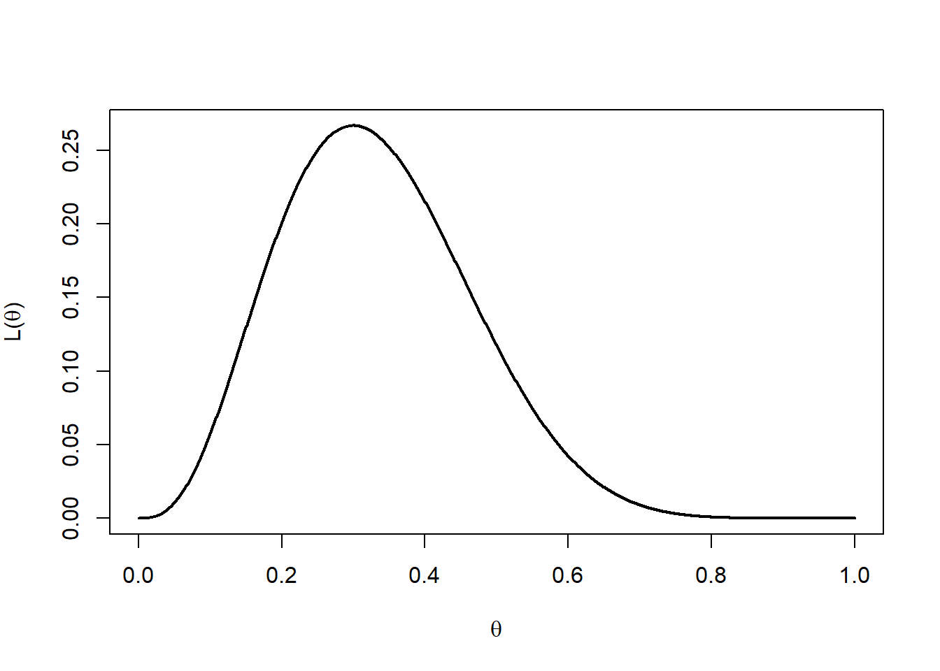
Figure 10.1: Likelihood function.

Take the derivative of \(L(\theta)\) (using the product rule):

\[\begin{align*} \frac{d L(\theta)}{d\theta} &= {m \choose x} x \theta^{x-1} (1-\theta)^{m-x} - {m \choose x} \theta^{x} (m-x) (1-\theta)^{m-x-1} \\[3pt] &= {m \choose x} \theta^{x-1} (1-\theta)^{m-x-1} \left[ x(1-\theta) - (m-x)\theta \right]. \end{align*}\]

Setting \(\frac{d L(\theta)}{d\theta} = 0\), we obtain

\[\left[ x(1-\theta) - (m-x)\theta \right] = 0.\]

Hence, \(\hat{\theta} = \frac{x}{m}\) is a possible value for the MLE of \(\theta\).

Since \(L(\theta)\) is a continuous function over \([0,1]\), the maximum must exist at either the stationary point or at one of the endpoints of the interval. Given, \(L(0) = 0\), \(L(1) = 0\), and \(L\left(\frac{x}{m}\right)>0\), it follows that \(\hat{\theta}=\frac{x}{m}\) is the MLE of \(\theta.\)

In the illustrative example, \(m=10\) and \(x=3\) giving \(\hat{\theta} = \frac{3}{10} =0.3\). In Figure 10.2 the MLE is marked on the plot of the likelihood function.

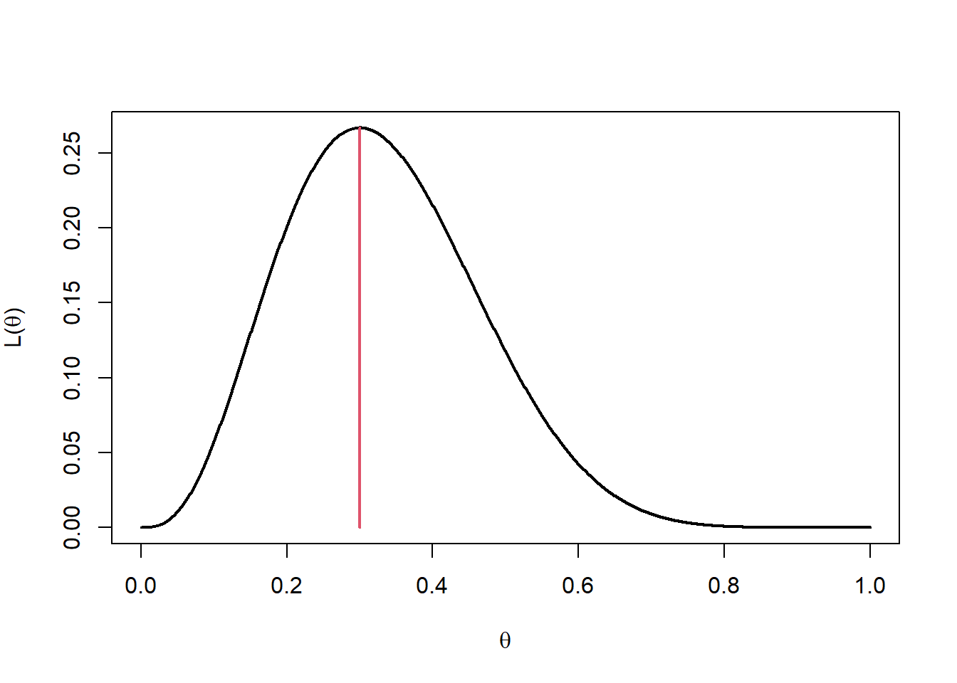
Figure 10.2: Likelihood function with MLE at 0.3.

It is easier to use the log-likelihood \(l(\theta)\) to derive the MLE.

We have that

\[l(\theta) = \log \left[ \binom{m}{x} \theta^x (1-\theta)^{m-x} \right] = \log \left[ \binom{m}{x}\right] + x \log \theta + (m-x) \log (1-\theta).\]

In the case \(m=10\) and \(x=3\) the likelihood becomes \(l(\theta) = \log 120 + 3 \log \theta + 7 \log (1-\theta)\) and this is illustrated in Figure 10.3.

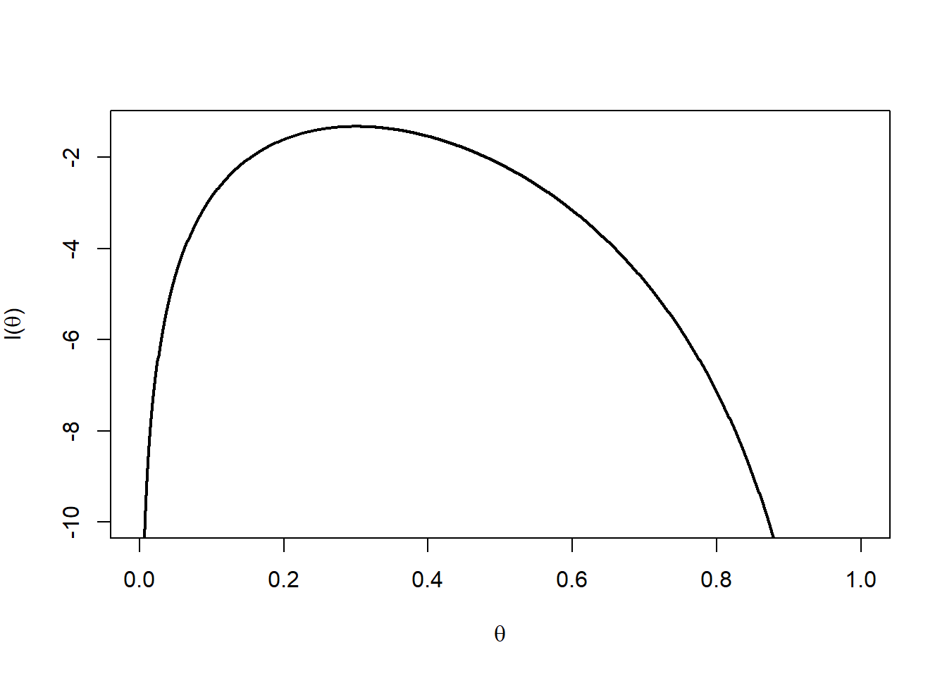
Figure 10.3: Log-likelihood function.

Take the derivative of \(l(\theta)\):

\[\begin{align*} \frac{d l(\theta)}{d\theta} &= 0 +\frac{x}{\theta} - \frac{m-x}{1-\theta} \\[3pt] &= \frac{x (1-\theta) - (m-x) \theta}{\theta (1-\theta)}. \end{align*}\] Setting \(\frac{d l(\theta)}{d\theta} = 0\), again requires solving \[\left[ x(1-\theta) - (m-x)\theta \right] = 0.\]

Hence, again giving \(\hat{\theta} = \frac{x}{m}\).

In the illustrative example, \(m=10\) and \(x=3\) giving \(\hat{\theta} = \frac{3}{10} =0.3\). In Figure 10.4 the MLE is marked on the plot of the likelihood function.

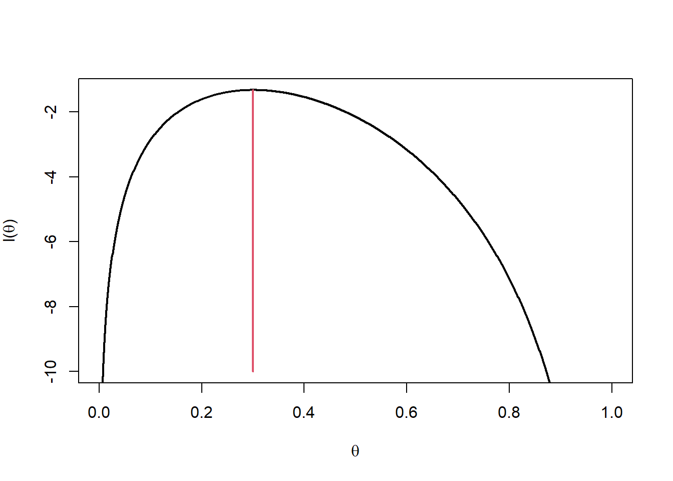
Figure 10.4: Log-likelihood function with MLE at 0.3.

The following R shiny app allows you to investigate the MLE for data from a geometric distribution, \(X \sim {\rm Geom} (p)\). The success probability of the geometric distribution can be varied from 0.01 to 1. The likelihood, log-likelihood and relative likelihood (likelihood divided by its maximum) functions can be plotted. Note that as the number of observations become large the likelihood becomes very small, and equal to, 0 to computer accuracy. You will observe that the likelihood function becomes more focussed about the MLE as the sample size increases. Also the MLE will generally be closer to the true value of \(p\) used to generate the data as the sample size increases.

MLE Geometric Distribution

Poisson MLE

Let \(X_1,X_2, \ldots, X_n\) be a random sample from a Poisson distribution with mean \(\lambda\). Find the MLE of \(\lambda\).

We have
\[\begin{align*} L(\lambda) &= p(x_1,x_2, \ldots, x_n | \lambda) \\[3pt] &= \frac{ \text{e}^{-n\lambda} \lambda^{\sum_{i=1}^n x_i}}{\prod_{i=1}^n x_i!}, \end{align*}\] where \(\lambda>0\). So, \[ l ( \lambda ) = -n \lambda + \sum\limits_{i=1}^n x_i \log \lambda - \log \prod\limits_{i=1}^n x_i!.\] Now \[ \frac{dl(\lambda)}{d\lambda} = -n + \frac{\sum_{i=1}^n x_i}{\lambda}. \] Setting \(\frac{dl(\lambda)}{d\lambda} =0\) and solving yields \[ \hat{\lambda} = \frac{\sum_{i=1}^n x_i}{n} = \bar{x}.\]

Since \(\frac{d^2 l(\lambda)}{d\lambda ^2} = \frac{-\sum_{i=1}^n x_i}{\lambda^2} < 0\), it follows that \(\hat{\lambda}=\bar{X}\) is a maximum and so is the MLE of \(\lambda\).

In both Exercise 1 and Examples 4, we note that terms in the likelihood which do not involve the parameter of interest play no role in the calculating of the MLE. For example, \(\binom{m}{x}\) in the binomial and \(\left[\prod\limits_{i=1}^n x_i!\right]^{-1}\) in the Poisson. Therefore it is sufficient to consider a function \(H(\theta)\) which is proportional to the likelihood, that is, there exists \(K >0\) such that \[ L(\theta) = K H(\theta) \qquad \mbox{for all } \theta. \] We write \(L(\theta) \propto H(\theta)\) and note that if \(h(\theta) = \log H (\theta)\), then
\[ l(\theta) = \log K + h (\theta)\] and
\[ \frac{d \;}{d \theta} l (\theta) = \frac{d \;}{d \theta} h (\theta).\]

MLE of mean of a Normal random variable

Let \(X_1,X_2, \ldots, X_n\) be a random sample of \(N(\theta,1)\) with mean \(\theta\). Find the MLE of \(\theta\) given observations \(x_1, x_2, \ldots, x_n\).

For each of the \(x_i\):
\[ f(x_i|\theta) = \frac{1}{\sqrt{2\pi}} \exp \left\{ -\frac{1}{2} \left(x_i-\theta\right)^2 \right\}.\] Thus: \[ L(\theta) = \left( 2 \pi\right)^{-n/2} \prod \limits_{i=1}^n \exp \left\{ -\frac{1}{2} \left(x_i-\theta\right)^2 \right\} \] and so, \[ L(\theta) \propto \prod \limits_{i=1}^n \exp \left\{ -\frac{1}{2} \left(x_i-\theta\right)^2 \right\} = \exp \left\{ -\frac{1}{2} \sum_{i=1}^n (x_i-\theta)^2\right\} \] and \[ l(\theta) = \log L(\theta) = -\frac{1}{2} \sum _{i=1}^n \left(x_i-\theta\right)^2 + \text{constant}.\] Hence \[ \frac{dl(\theta)}{d\theta} = \sum _{i=1}^n (x_i-\theta) = 0\] gives the stationary point of the likelihood, with \[\begin{equation} \hat{\theta} = \frac{\sum x_i}{n} = \bar{x}, \tag{10.1} \end{equation}\] It is easily verified that \(\hat{\theta}\) given in (10.1) is a maximum since \[ \frac{d^2 l(\theta)}{d\theta^2} = -n < 0 .\]

So \(\hat{\theta}= \bar{x}\) is the MLE of \(\theta\).

In Exercise 1, Example 4 and Example 5 the maximum likelihood estimators correspond with the method of moment estimators. In Exercise 2 we consider a situation where the maximum likelihood estimator is very different from the method of moments estimator.

MLE for Uniform random variables

Let \(U_1,U_2, \ldots, U_n\) be i.i.d. samples of \(U[0,\theta]\). Given observations \(u_1, u_2, \ldots, u_n\):

1. Find the MLE of \(\theta\).
   
2. Find the method of moments estimator of \(\theta\).

Attempt Exercise 2: MLE for Uniform random variables and then watch Video 18 for the solutions.

We will data \(\mathbf{u}= (u_1, u_2, \ldots, u_5)= (1.30,2.12,2.40,0.98,1.43)\) as an illustrative example. These 5 observations were simulated from \(U(0,3)\).

Video 18: MLE for Uniform random variables

Alternatively worked solutions are provided:

Solution to Exercise 2: MLE for Uniform random variables

1. If \(U_i \sim U[0,\theta]\), then its p.d.f. is given by
   \[f(u|\theta) = \begin{cases} \frac{1}{\theta}, & \text{if } 0 \leq u \leq \theta, \\[3pt] 0, & \text{otherwise.} \end{cases}\] Note that if \(\theta< u_i\) for some \(i\), then \(L(\theta)=0\). Since \(L(\theta)\) is always positive and we want to maximise L, we can assume \(0 \leq u_i \leq \theta\) for all \(i=1,\dots,n\), then \[L(\theta) = \prod_{i=1}^n f(u_i|\theta) = \prod_{i=1}^n \frac{1}{\theta} = \frac{1}{\theta^n}.\] Hence, \(L(\theta)\) is a decreasing function of \(\theta\) and its maximum must exist at the smallest value that \(\theta\) can obtain. Since \(\theta > \max \{u_1,u_2,\dots,u_n\}\), the MLE of \(\theta\) is \(\hat{\theta} = \max \{u_1,u_2,\dots,u_n\}\).

Figure 10.5 shows the likelihood function \(L(\theta)\) using the data \(\mathbf{u}= (1.30,2.12,2.40,0.98,1.43)\).

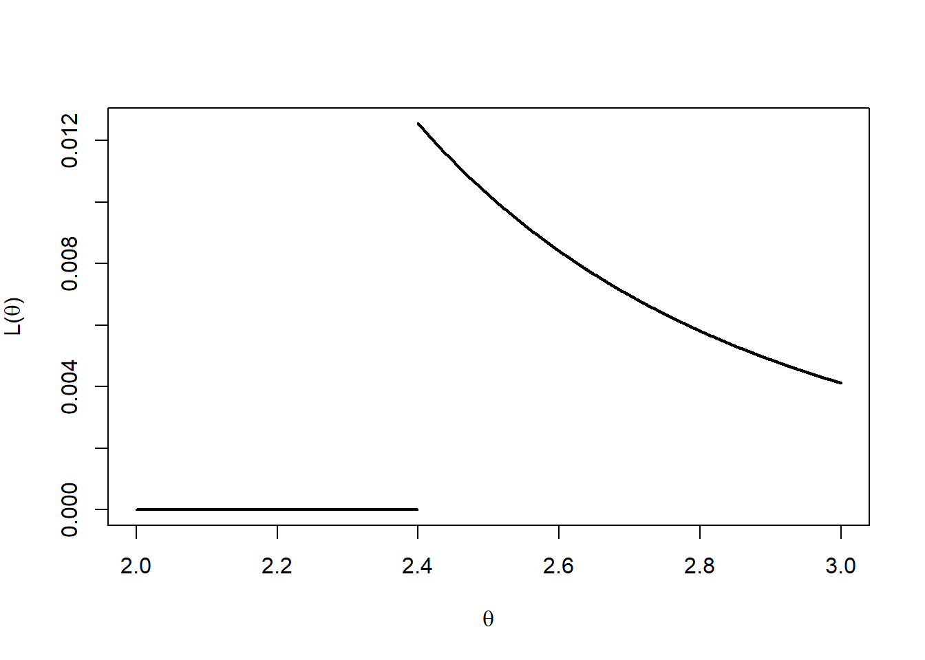
Figure 10.5: Likelihood function for u = (1.30,2.12,2.40,0.98,1.43).

2. By comparison the method of moments estimator, \(\check{\theta}\), of \(\theta\) uses \(E[U]= \frac{0 +\theta}{2}\) and hence is given by \[ \check{\theta} = 2 \bar{u}. \] Note that if \(2 \bar{u} < \max \{u_1,u_2,\dots,u_n\}\) then \(\check{\theta}\) will not be consistent with the data, i.e. \(L(\check{\theta})=0\).

To observe the difference between the MLE and the method of moments estimator, using \(\mathbf{u}= (1.30,2.12,2.40,0.98,1.43)\):

• MLE: \(\hat{\theta} = \max \{1.30,2.12,2.40,0.98,1.43 \} =2.40\);
  
• Method of Moments: \(\check{\theta} =2 \bar{u} = 2 (1.646) =3.292\).
  

10.4 Comments on the Maximum Likelihood Estimator

The following points on the maximum likelihood estimator are worth noting:

1. When finding the MLE you want to maximise the likelihood function. However it is often more convenient to maximise the log likelihood function instead. Both functions will be maximised by the same parameter values;
   
2. MLEs may not exist, and if they do, they may not be unique;
   
3. The likelihood function is NOT the probability distribution for \(\theta\). The correct interpretation of the likelihood function is that it is the probability of obtaining the observed data if \(\theta\) were the true value of the parameter. We assume \(\theta\) is an unknown constant, not a random variable. In Bayesian statistics we will consider the parameter to be random;
   
4. The MLE has some nice large sample properties, including consistency, asymptotic normality and other optimality properties;
   
5. The MLE can be used for non-independent data or non-identically distributed data as well;
   
6. Often the MLE cannot be found using calculus techniques and must be found numerically. It is often useful, if we can, to plot the likelihood function to find good starting points to find the MLE numerically;
   
7. The MLE satisfies a useful invariance property. Namely, if \(\phi = h(\theta)\), where \(h(\theta)\) is a one-to-one function of \(\theta\), then the MLE of \(\phi\) is given by \(\hat{\phi} = h (\hat{\theta})\). For example, if \(\phi = \frac{1}{\theta}\) and \(\hat{\theta}=\bar{X}\) then \(\hat{\phi} = \frac{1}{\hat{\theta}} = \frac{1}{\bar{X}}\).

Student Exercises

Attempt the exercises below.

Question 1.

Let \(X_1, X_2, \dots, X_n\) be independent random variables, each with pdf \[ f(x | \theta) = \theta^2 x \exp(-\theta x),\] for \(x > 0\). Use the method of moments to determine an estimator of \(\theta\).

Remember that if \(X \sim \text{Gamma}(\alpha,\beta)\) then \(E[X]=\alpha/\beta\).

Solution to Question 1.

The distribution is \({\rm Gamma} (\alpha, \beta)\) with \(\alpha = 2\) and \(\beta = \theta\) since
\[ \frac {{\beta}^{\alpha} x^{\alpha - 1} e^{-\beta x}}{\Gamma (\alpha)} = \frac {{\theta}^{2} x^{2 - 1} e^{-\theta x}}{\Gamma (2)} = {\theta}^2 x e^{-\theta x}. \] For the \({\rm Gamma} (\alpha, \beta)\) distribution
\[E[X] = \frac {\alpha}{\beta} = \frac {2}{\theta}.\] Alternatively this can be obtained directly using integration by parts.
By the method of moments, \[ E[X]= \frac {\alpha}{\beta} = \frac {2}{\theta} = \bar{x} \qquad \Rightarrow \qquad \theta = \frac {2}{\bar{x}}.\]

Question 2.

Let \(X_1, X_2, \dots, X_n\) be a random sample from the distribution with p.d.f. \[ f(x|\theta) = \theta e^{-(x-1)\theta}, \qquad x>1,\]

where \(\theta > 0\) is an unknown parameter. Find the MLE of \(\theta\).

Solution to Question 2.

The likelihood is \[\begin{eqnarray*} L(\theta) = \prod_{i=1}^n f(x_i | \theta) = \prod _{i=1}^n \theta e^{-(x_i-1)\theta} &=& \theta^n \exp \left\{ - \sum_{i=1}^n (x_i-1)\theta \right\} \\ &=& \theta^n \exp \left\{ - \left( \sum_{i=1}^n x_i-n \right) \theta \right\}. \end{eqnarray*}\] Thus \[ l(\theta) = \log L(\theta) = n \log \theta - \left( \sum_{i=1}^n x_i-n \right) \theta, \] so \[ l'(\theta)=\frac{n}{\theta}- \sum_{i=1}^n x_i+n.\] For a stationary point, \[\begin{eqnarray*} l'(\theta) = 0 \qquad &\Longleftrightarrow& \qquad \frac{n}{\theta}-\sum_{i=1}^n x_i+n=0 \\ \qquad &\Longleftrightarrow& \qquad \theta = \frac{n}{\sum_{i=1}^n x_i-n} = \frac{1}{\bar{x}-1}. \end{eqnarray*}\] This corresponds to a maximum since \[ l''(\theta)=-\frac{n}{\theta ^2}<0. \]

Thus the MLE of \(\theta\) is \(\hat{\theta}=\frac{1}{\bar{x}-1}\).

Question 3.

1. Let \(X_1, X_2, \dots, X_n\) be a random sample from the distribution having pdf \[ f(x|\theta) = \frac{1}{2} (1+ \theta x), \qquad -1<x<1,\] where \(\theta \in (-1,1)\) is an unknown parameter. Show that the method of moments estimator for \(\theta\) is \[\tilde{\theta}_1 = 3 \bar{X}\] where \(\bar{X} = \frac{1}{n} \sum_{i=1}^n X_i.\)
   
2. Suppose instead that it is observed only whether a given observation is positive or negative. For \(i=1,2,\dots,n\), let
   \[ Y_i = \begin{cases} 1 & \text{if } X_i \geq 0 \\ 0 & \text{if } X_i < 0. \end{cases} \] Show that the method of moments estimator for \(\theta\) based on \(Y_1, Y_2, \dots, Y_n\) is
   \[\tilde{\theta}_2 = 4 \bar{Y} - 2,\] where \(\bar{Y} = \frac{1}{n} \sum_{i=1}^n Y_i.\)
   
3. Justifying your answers,

1. which, if either, of the estimators \(\tilde{\theta}_1\) and \(\tilde{\theta}_2\) are unbiased?
   
2. which of the estimators \(\tilde{\theta}_1\) and \(\tilde{\theta}_2\) is more efficient?
   
3. which, if either, of the estimators \(\tilde{\theta}_1\) and \(\tilde{\theta}_2\) are mean-square consistent?

Solution to Question 3.

1. Since,
   \[ E[X_1] = \int_{-1}^{1} \frac{x}{2}(1+ \theta x) dx = \left[ \frac{x^2}{4} + \theta \frac{x^3}{6} \right]_{-1}^1 = \frac{\theta}{3}, \] the method of moments estimator is obtained by solving \(\bar{X} = \frac{\theta}{3}\) yielding, \(\tilde{\theta}_1 = 3\bar{X}\).
   
2. First note that,
   \[ P(X_1 > 0) = \int_0^1 \frac{1}{2} (1+\theta x) dx = \left[ \frac{x}{2} + \theta \frac{x^2}{4} \right]_0^1 = \frac{1}{2} \left(1+\frac{\theta}{2}\right).\] Thus,
   \[ E[Y_1] = P(X_1 > 0) = \frac{1}{2} \left(1+\frac{\theta}{2}\right), \] so, \(\bar{Y} = \frac{1}{2} \left(1+\frac{\theta}{2}\right)\), yielding,
   \[ \tilde{\theta}_2 = 4\bar{Y} - 2.\]

1. Both estimators are unbiased. \[ E[\tilde{\theta}_1] = E \left[ \frac{3}{n} \sum_{i=1}^n X_i \right] = \frac{3}{n} \sum_{i=1}^n E[X_i] = \frac{3}{n} n \frac{\theta}{3} = \theta, \] so \(\tilde{\theta}_1\) is unbiased.
   \[ E[\tilde{\theta}_2] = E \left[ \frac{4}{n} \sum_{i=1}^n Y_i - 2 \right] = \frac{4}{n} \sum_{i=1}^n E[Y_i] - 2 = \frac{4}{n} n \frac{1}{2} \left(1+ \frac{\theta}{2}\right) - 2 = \theta, \] so \(\tilde{\theta}_2\) is unbiased.
   
2. \[ var(\tilde{\theta}_1) = var\left( \frac{3}{n} \sum_{i=1}^n X_i \right) = \frac{9}{n^2} \sum_{i=1}^n var(X_i) = \frac{9}{n} var(X_1). \] Now,
   \[ E[X_1^2] = \int_{-1}^1 \frac{x^2}{2} (1+\theta x) dx = \left[ \frac{x^3}{6} + \theta \frac{x^4}{8} \right]_{-1}^1 = \frac{1}{3}. \] Thus,
   \[ var(X_1) = \frac{1}{3} - \frac{\theta^2}{9} = \frac{1}{9}(3-\theta^2), \] so,
   \[ var(\tilde{\theta}_1) = \frac{1}{n}(3-\theta^2). \] Similarly,
   \[ var(\tilde{\theta}_2) = var(4\bar{Y} -2) = 16 var(\bar{Y}) = \frac{16}{n} var(Y_1). \] Now \(Y_1 \sim \text{Bin}\left(1,\frac{1}{2}\left(1+\frac{\theta}{2}\right) \right)\) so,
   \[ var(Y_1) = \frac{1}{2}\left(1+\frac{\theta}{2}\right)\frac{1}{2}\left(1-\frac{\theta}{2}\right) = \frac{1}{4}\left(1-\frac{\theta^2}{4}\right) = \frac{1}{16}(4-\theta^2), \] thus,
   \[ var(\tilde{\theta}_2) = \frac{1}{n}(4-\theta^2). \] Hence, \(var(\tilde{\theta}_1) < var(\tilde{\theta}_2)\), so \(\tilde{\theta}_1\) is more efficient than \(\tilde{\theta}_2\).
   
3. Since \(\tilde{\theta}_i\) is unbiased, \(MSE(\tilde{\theta}_i) = var(\tilde{\theta}_i)\) for \(i=1,2\). Thus
   \[MSE(\tilde{\theta}_1) = \frac{1}{n}(3-\tilde{\theta}_1^2) \rightarrow 0 \qquad \mbox{ as } \; n \rightarrow \infty.\] So \(\tilde{\theta}_1\) is consistent.
   Also, \[MSE(\tilde{\theta}_2) = \frac{1}{n}(4-\tilde{\theta}_2^2) \rightarrow 0 \qquad \mbox{ as } \; n \rightarrow \infty.\] So \(\tilde{\theta}_2\) is consistent.