Chapter 7 Central Limit Theorem and law of large numbers

7.1 Introduction

In this Section we will show why the Normal distribution, introduced in Section 5.7, is so important in probability and statistics. The central limit theorem states that under very weak conditions (almost all probability distributions you will see will satisfy them) the sum of $n$ i.i.d. random variables, $S_n$, will converge, appropriately normalised to a standard Normal distribution as $n \to \infty$. For finite, but large $n (\geq 50)$, we can approximate $S_n$ by a normal distribution and the normal distribution approximation can be used to answer questions concerning $S_n$. In Section 7.2 we present the Central Limit Theorem and apply it to an example using exponential random variables. In Section 7.3 we explore how a continuous distribution (the Normal distribution) can be used to approximate sums of discrete distributions. Finally, in Section 7.4, we present the Law of Large Numbers which states that the uncertainty in the sample mean of $n$ observations $S_n/n$ decreases as $n$ increases and converges to the population mean $\mu$. Both the Central Limit Theorem and the Law of Large Numbers will be important moving forward when considering statistical questions.

7.2 Statement of Central Limit Theorem

Before stating the Central Limit Theorem, we introduce some notation.

A sequence of random variables $Y_1, Y_2, \ldots$ are said to converge in distribution to a random variable $Y$, if for all $y \in \mathbb{R}$, $$P(Y_n \leq y) \rightarrow P(Y \leq y) \qquad \qquad \mbox{ as } \; n \to \infty.$$

We write $Y_n \xrightarrow{\quad D \quad} Y$ as $n \to \infty$.

Central Limit Theorem.
Let $X_1,X_2,\dots,X_n$ be independent and identically distributed random variables (i.e. a random sample) with finite mean $\mu$ and variance $\sigma^2$. Let $S_n = X_1 + \cdots + X_n$. Then $$\frac{S_n - n\mu}{\sigma \sqrt{n}} \xrightarrow{\quad D \quad} N(0,1).$$

The central limit theorem is equivalent to $$\frac{\bar{X} - \mu}{\sigma/\sqrt{n}} \xrightarrow{\quad D \quad} N(0,1).$$

where $\bar{X} = \frac{1}{n} \sum_{i=1}^n X_i$ is the mean of the distributions $X_1, X_2, \ldots , X_n$.

Therefore, we have that for large $n$, $$S_n \approx N(n \mu, n \sigma^2)$$ and $$\bar{X} \approx N\left(\mu, \frac{\sigma^2}{n} \right).$$

Suppose $X_1,X_2,\dots,X_{100}$ are i.i.d. exponential random variables with parameter $\lambda=4$.

1. Find $P(S_{100} > 30)$.
   
2. Find limits within which $\bar{X}$ will lie with probability $0.95$.
   

1. Since $X_1,X_2,\dots,X_{100}$ are i.i.d. exponential random variables with parameter $\lambda=4$, $E\left[X_i\right]=\frac{1}{4}$ and $var(X_i) = \frac{1}{16}$. Hence,

   $$\begin{align*} E \left[ S_{100} \right] &= 100 \cdot \frac{1}{4} = 25; \\ var(S_{100}) &= 100 \cdot \frac{1}{16} = \frac{25}{4}. \end{align*}$$

   Since $n=100$ is sufficiently big, $S_{100}$ is approximately normally distributed by the central limit theorem (CLT). Therefore,

   $$\begin{align*} P(S_{100} > 30) &= P \left( \frac{S_{100}-25}{\sqrt{\frac{25}{4}}} > \frac{30-25}{\sqrt{\frac{25}{4}}} \right) \\ &\approx P( N(0,1) >2) \\ &= 1 - P( N(0,1) \leq 2) \\ &= 0.0228. \end{align*}$$

   Given that $S_{100} = \sum_{i=1}^{100} X_i \sim {\rm Gamma} (100,4)$, we can compute the exactly $P(S_{100} >30) = 0.0279$, which shows that the central limit theorem gives a reasonable approximation.

2. Since $X_1,X_2,\dots,X_{100}$ are i.i.d. exponential random variables with parameter $\lambda=4$, $E\left[X_i\right]=\frac{1}{4}$ and $var (X_i) = \frac{1}{16}$. Therefore, $E\left[\bar{X}\right] = \frac{1}{4}$ and $var(\bar{X}) = \frac{1/16}{100}$.
   Since $n=100$, $\bar{X}$ will be approximately normally distributed by the CLT, hence

   $$\begin{align*} 0.95 &= P(a < \bar{X} < b) \\ &= P \left( \frac{a-1/4}{\sqrt{1/1600}} < \frac{\bar{X}-1/4}{\sqrt{1/1600}} < \frac{b-1/4}{\sqrt{1/1600}} \right) \\ &\approx P \left( \frac{a-1/4}{\sqrt{1/1600}} < N(0,1) < \frac{b-1/4}{\sqrt{1/1600}} \right). \\ \end{align*}$$

   There are infinitely many choices for $a$ and $b$ but a natural choice is $P(\bar{X}<a) = P (\bar{X}>b) = 0.025$. That is, we choose $a$ and $b$ such that there is equal chance that $\bar{X}$ is less than $a$ or greater than $b$. Thus if for $0 < q< 1$, $z_q$ satisfies $P(Z < z_q)=q$, we have that
   

   $$\begin{align*} \frac{a-1/4}{\sqrt{1/1600}} &= z_{0.025} = -1.96, \\ \frac{b-1/4}{\sqrt{1/1600}} &= z_{0.975} = 1.96. \end{align*}$$

   Hence,
   

   $$\begin{align*} a &= 0.25 - 1.96 \frac{1}{40} = 0.201, \\ b &= 0.25 + 1.96 \frac{1}{40} = 0.299. \end{align*}$$

7.3 Central limit theorem for discrete random variables

The central limit theorem can be applied to sums of discrete random variables as well as continuous random variables. Let $X_1, X_2, \ldots$ be i.i.d. copies of a discrete random variable $X$ with $E[X] =\mu$ and $var(X) = \sigma^2$. Further suppose that the support of $X$ is in the non-negative integers $\{0,1, \ldots \}$. (This covers all the discrete distributions, we have seen, binomial, negative binomial, Poisson and discrete uniform.)

Let $Y_n \sim N(n \mu, n \sigma^2)$. Then the central limit theorem states that for large $n$, $S_n \approx Y_n$. However, there will exist $x \in \{0,1,\ldots \}$ such that
$$P(S_n =x) >0 \qquad \qquad \mbox{but} \qquad \qquad P(Y_n =x) =0.$$ The solution is that we approximate
$$P(S_n =x) \qquad \qquad \mbox{by} \qquad \qquad P(x - 0.5 <Y_n \leq x+0.5) =0.$$

This is known as the continuity correction.

Suppose that $X$ is a Bernoulli random variable with $P(X=1)=0.6 (=p)$, so $E[X]=0.6$ and $var(X) =0.6 \times (1-0.6) =0.24$. Then $$S_n = \sum_{i=1}^n X_i \sim {\rm Bin} (n, 0.6).$$

For $n=100$, $S_{100} \sim {\rm Bin} (100, 0.6)$ can be approximated by $Y\sim N(60,24) (=N(np,np(1-p)))$, see Figure 7.1.

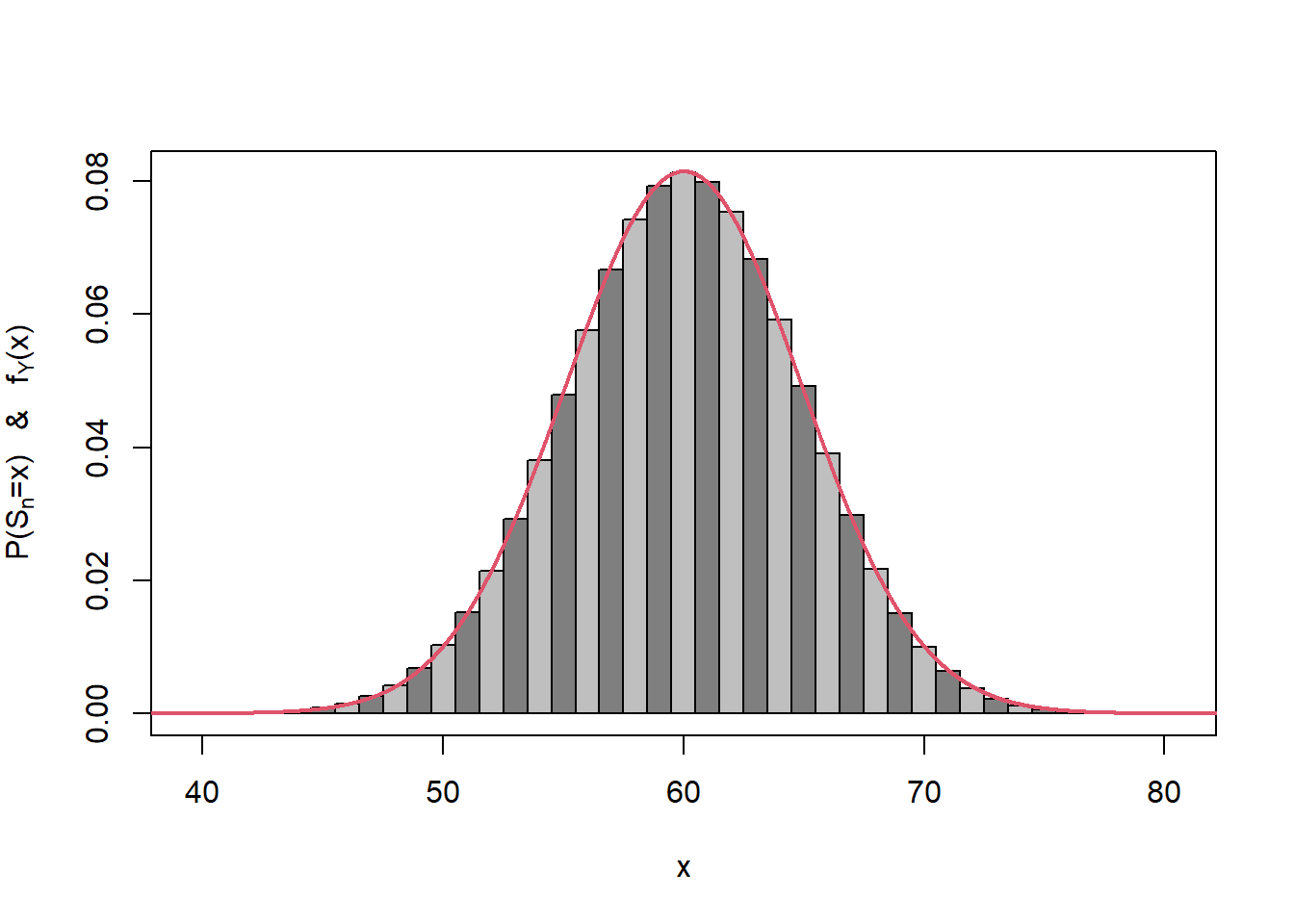
Figure 7.1: Central limit theorem approximation for the binomial.

We can see the approximation in Figure 7.1 in close-up for $x=54$ to $56$ in Figure 7.2.

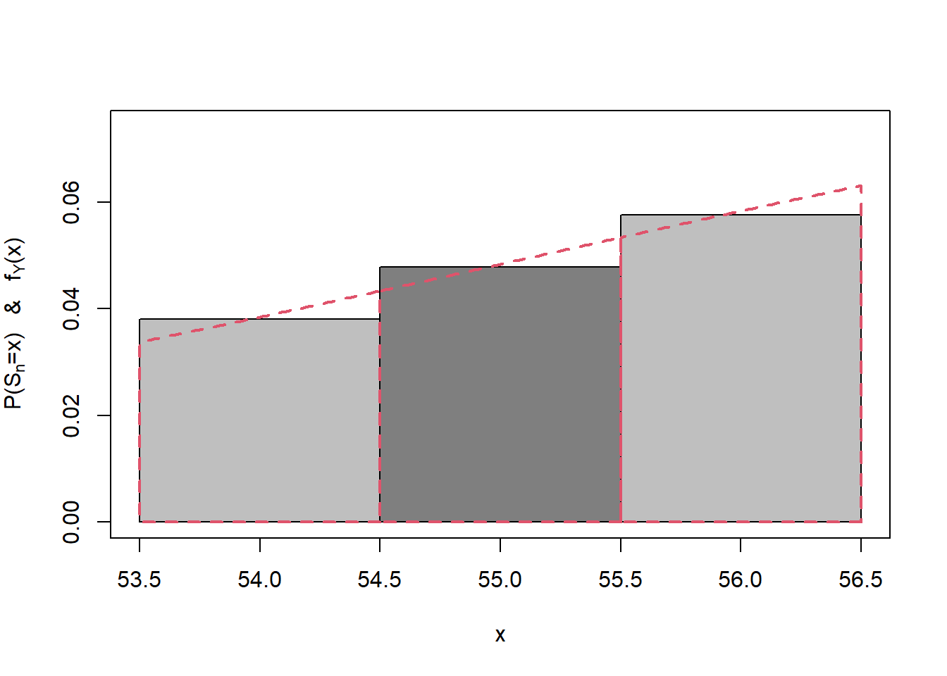
Figure 7.2: Central limit theorem approximation for the binomial for x=54 to 56.

7.4 Law of Large Numbers

We observed that $$\bar{X} \approx N\left(\mu, \frac{\sigma^2}{n} \right),$$ and the variance is decreasing as $n$ increases.

Given that $$var (S_n) = var \left(\sum_{i=1}^n X_i \right) = \sum_{i=1}^n var \left( X_i \right) = n \sigma^2,$$ we have in general that $$var (\bar{X}) = var \left(\frac{S_n}{n} \right) = \frac{1}{n^2} var (S_n) = \frac{\sigma^2}{n}.$$

A random variable $Y$ which has $E[Y]=\mu$ and $var(Y)=0$ is the constant, $Y \equiv \mu$, that is, $P(Y=\mu) =1$. This suggests that as $n \to \infty$, $\bar{X}$ converges in some sense to $\mu$. We can make this convergence rigorous.

A sequence of random variables $Y_1, Y_2, \ldots$ are said to converge in probability to a random variable $Y$, if for any $\epsilon >0$, $$P(|Y_n - Y|> \epsilon) \to 0 \qquad \qquad \mbox{ as } \; n \to \infty.$$ We write $Y_n \xrightarrow{\quad p \quad} Y$ as $n \to \infty$.

We will often be interested in convergence in probability where $Y$ is a constant.

A useful result for proving convergence in probability to a constant $\mu$ is Chebychev’s inequality. Chebychev’s inequality is a special case of the Markov inequality which is helpful in bounding probabilities in terms of expectations.

Chebychev’s inequality.
Let $X$ be a random variable with $E[X] =\mu$ and $var(X)=\sigma^2$. Then for any $\epsilon >0$, $$P(|X - \mu| > \epsilon) \leq \frac{\sigma^2}{\epsilon^2}.$$

Law of Large Numbers.
Let $X_1, X_2, \ldots$ be i.i.d. according to a random variable $X$ with $E[X] = \mu$ and $var(X) =\sigma^2$. Then $$\bar{X} = \frac{1}{n} \sum_{i=1}^n X_i \xrightarrow{\quad p \quad} \mu \qquad \qquad \mbox{ as } \; n \to \infty.$$

First, note that $$E[\bar{X}] = E \left[ \frac{1}{n} \sum_{i=1}^n X_i \right]= \frac{1}{n} \sum_{i=1}^n E \left[ X_i \right] = \frac{1}{n} (n \mu) = \mu.$$ For any $\epsilon >0$, we have by Chebychev’s inequality that
$$P(|\bar{X}- \mu| > \epsilon) \leq \frac{1}{\epsilon^2} var (\bar{X}) = \frac{\sigma^2}{n \epsilon^2} \to 0 \qquad \qquad \mbox{ as } n \to \infty,$$

and the Theorem follows.

Figure 7.3: Dice picture.

Central limit theorem for dice

Let $D_1, D_2, \ldots$ denote the outcomes of successive rolls of a fair six-sided dice.

Let $S_n = \sum_{i=1}^n D_i$ denote the total score from $n$ rolls of the dice and let $M_n = \frac{1}{n} S_n$ denote the mean score from $n$ rolls of the dice.

1. What is the approximate distribution of $S_{100}$?
   
2. What is the approximate probability that $S_{100}$ lies between $330$ and $380$, inclusive?
   
3. How large does $n$ need to be such that $P(|M_n - E[D]|>0.1) \leq 0.01$?
   

Attempt Exercise 1 and then watch Video 15 for the solutions.

Video 15: Central limit theorem for dice

Alternatively the solutions are available:

Solution to Exercise 1

Note that $D_1$ is a discrete uniform distribution with probability mass function $$P(D_1 =x) = \left\{ \begin{array}{ll} \frac{1}{6} \qquad \qquad & x=1,2,\ldots, 6, \\ 0 & \mbox{otherwise}. \end{array} \right.$$

Then $E[D_1] = \frac{7}{2} =3.5$ and $Var (D_1) = \frac{35}{12}$.

1. Since the rolls of the dice are independent,
   

   $$\begin{eqnarray*} E[S_{100}] &=& E \left[ \sum_{i=1}^{100} D_i \right] = \sum_{i=1}^{100}E \left[ D_i \right] \\ &=& 100 E[D_1] = 350. \end{eqnarray*}$$

   and

   $$\begin{eqnarray*} var(S_{100}) &=& var \left( \sum_{i=1}^{100} D_i \right) = \sum_{i=1}^{100}var \left( D_i \right) \\ &=& 100 var(D_1)= \frac{875}{3}. \end{eqnarray*}$$

   Thus by the central limit theorem, $S_{100} \approx Y \sim N \left(350, \frac{875}{3} \right)$.

2. Using the CLT approximation above, and the continuity correction
   

   $$\begin{eqnarray*}P(330 \leq S_{100} \leq 380) &\approx& P(329.5 \leq Y \leq 380.5) \\ &=& P(Y \leq 380.5) - P(Y \leq 329.5) \\ &=& 0.9629 - 0.115 = 0.8479. \end{eqnarray*}$$

   If using Normal tables, we have that
   

   $$P\left( Y \leq 380.5 \right) = P \left( Z = \frac{Y-350}{\sqrt{875/3}} \leq \frac{380.5-350}{\sqrt{875/3}} \right) = \Phi (1.786)$$

   and
   

   $$P\left( Y \leq 329.5 \right) = P \left( Z = \frac{Y-350}{\sqrt{875/3}} \leq \frac{329.5-350}{\sqrt{875/3}} \right) = \Phi (-1.200).$$

3. Using the Central Limit Theorem, $M_n \approx W_n \sim N \left(\frac{7}{2}, \frac{35}{12 n} \right)$.
   We know by the law of large numbers that $M_n \xrightarrow{\quad p \quad} \frac{7}{2}$ as $n \to \infty$, but how large does $n$ need to be such that there is a $99\%$ (or greater) chance of $M_n$ being within $0.1$ of $3.5$?
   Using the approximation $W_n$, we want:
   

   $$P \left(\left| W_n - \frac{7}{2} \right| > 0.1 \right) \leq 0.01.$$

   Now
   

   $$\begin{eqnarray*} P \left(\left| W_n - \frac{7}{2} \right| > 0.1 \right) &=& P(3.4 \leq W_n \leq 3.6) \\ &= & P \left( \frac{3.4 -3.5}{\sqrt{35/(12n)}} \leq Z \leq \frac{3.6 -3.5}{\sqrt{35/(12n)}} \right) \\ &=& P \left( - 0.058554 \sqrt{n} < Z < 0.58554 \sqrt{n} \right) = P(|Z| > 0.058554 \sqrt{n}). \end{eqnarray*}$$

   Consider $P(|Z| > 0.058554 \sqrt{n}) =0.01$.
   Note that
   

   $$P(|Z| >c) =\alpha \hspace{1cm} \Leftrightarrow \hspace{1cm} P (Z >c) = \frac{\alpha}{2} \hspace{1cm} \Leftrightarrow \hspace{1cm} P (Z \leq c) = 1-\frac{\alpha}{2}.$$

   We have $\alpha =0.01$, and using qnorm function in R qnorm(0.995) gives $c =$ 2.5758293.
   Therefore

   $$P(|Z| > 0.058554 \sqrt{n}) =0.01 = P(|Z|>2.5758),$$ or equivalently $$0.058554 \sqrt{n} = 2.5758 \hspace{1cm} \Rightarrow \hspace{1cm} \sqrt{n} = 43.99 \hspace{1cm} \Rightarrow \hspace{1cm} n = 1935.2.$$

   Given that we require $n \geq 1935.2$, we have that $n=1936$.
   

Task: Lab 4

Attempt the R Markdown file for Lab 4:
Lab 4: Convergence and the Central Limit Theorem

Student Exercises

Attempt the exercises below.

Question 1.

Let $X_1, X_2, \dots, X_{25}$ be independent Poisson random variables each having mean 1. Use the central limit theorem to approximate $$P\left( \sum_{i=1}^{25} X_i > 20 \right).$$

Solution to Question 1.

Let $X=\sum_{i=1}^{25}X_i$. Then, $E[X]=25$ and $var(X)=25$. By the central limit theorem, $X\approx Y \sim N(25,5^2)$ $$\begin{eqnarray*} P(X>20) \approx P(Y>20.5) = 0.8159. \end{eqnarray*}$$ Converting to a standard normal distribution, $Z \sim N(0,1)$. $$\begin{eqnarray*} P(Y >20.5) &=& P \left( Z=\frac{Y-25}{5} > \frac{20.5-25}{5} \right) \\ &=& P(Z>-0.9) =P(Z<0.9) = `r round(pnorm(0.9),4)`. \end{eqnarray*}$$

Note that the final step comes from the symmetry of the normal distribution.

For comparison, since $X \sim {\rm Po} (25)$, we have that $P(X >20) = `r 1-round(ppois(20,25),4)`$.

Question 2.

The lifetime of a Brand X TV (in years) is an exponential random variable with mean 10. By using the central limit theorem, find the approximate probability that the average lifetime of a random sample of 36 TVs is at least 10.5.

Solution to Question 2.

Let $X_i$ denote the lifetime of the $i^{th}$ TV in the sample, $i=1, 2 \ldots, 36$. Then (from the lecture notes) we know that $E[X_i] = 10$, $var(X_i) = 100$.

The sample mean is $\bar{X} = (X_1 + \ldots X_{36})/36$.

Using the central limit theorem, $X_1 + \ldots + X_{36} \approx N(360, 3600)$, so $$\bar{X} \approx N \left(\frac{360}{36}, \frac{3600}{36^2} \right) = N(10, 2.778).$$ Thus $$\begin{eqnarray*} P(\bar{X} > 10.5) &=& P \left(\frac{\bar{X} - 10}{\sqrt{2.778}} > \frac{10.5-10}{\sqrt{2.778}} \right) \\ &\approx& P(Z > 0.3) \end{eqnarray*}$$

where $Z \sim N(0,1)$. Thus the required probability is approximately $P(Z > 0.3) = 1 - \Phi(0.3) = `r round(pnorm(-0.3),4)`$.

Question 3.

Prior to October 2015, in the UK National Lottery gamblers bought a ticket on which they mark six different numbers from $\{ 1,2,\ldots,49 \}$. Six balls were drawn uniformly at random without replacement from a set of $49$ similarly numbered balls. A ticket won the jackpot if the six numbers marked are the same as the six numbers drawn.

1. Show that the probability a given ticket won the jackpot is $1/13983816$.
   
2. In Week 9 of the UK National Lottery $69,846,979$ tickets were sold and there were $133$ jackpot winners. If all gamblers chose their numbers independently and uniformly at random, use the central limit theorem to determine the approximate distribution of the number of jackpot winners that week. Comment on this in the light of the actual number of jackpot winners.

Solution to Question 3.

1. There are $\binom{49}{6}=13,983,816$ different ways of choosing 6 distinct numbers $1,2,\ldots,49$, so the probability a ticket wins the jackpot if $1/13983816$.
   
2. Let $X$ be the number of jackpot winners in Week 9 if gamblers chose their numbers independently and uniformly at random. Then
   $$X \sim{\rm Bin} \left( 69,846,979, \frac{1}{13,989,816} \right) = {\rm Bin} (n,p), \text{ say}.$$ Then to 4 decimal places $E[X] =n p = 4.9927$ and $var(X)=np(1-p)=4.9927$.
   Hence, by the central limit theorem, $$X \approx N(4.9927,4.9927).$$

Given the Central Limit Theorem the probability of at least 133 jackpot winners is, using the continuity correction, $$\begin{align*} P(X \geq 133) &\approx P \left( \frac{X-4.9927}{\sqrt{4.9927}} \geq \frac{132.5-4.9927}{\sqrt{4.9927}} \right)\\ &= P (Z \geq 57.065), \end{align*}$$

where $Z \sim N(0,1)$. This probability is small, so there is very strong evidence that the gamblers did not choose their numbers independently and uniformly at random.