7.3 (R-) Workflow for Text Analysis

Retrieve data / data collection
Data manipulation / Corpus pre-processing
Vectorization: Turning Text into a Matrix (DTM/DFM)
Analysis
Validation and Model Selection
Visualization and Model Interpretation

7.3.1 Data collection

use existing corpora
- R: {gutenbergr}: contains more than 60k book transcripts
- R: {quanteda.corpora}: provides multiple corpora; see here for a overview
- R: {topicmodels}: contains Associated Press data (2246 news articles mostly from around 1988)
- search for datasets, see e.g. this list
collect new corpora
- electronic sources (APIs, Web Scraping), e.g. twitter, wikipedia, transcripts of all german electoral programs
- undigitized text, e.g. scans of documents
- data from interviews, surveys and/or experiments
consider relevant applications to turn your data into text format (speech-to-text recognition (google API), pdf-to-text, OCR))

7.3.2 Data manipulation: Basics (1)

text data is different from “structured” data (e.g., a set of rows and columns)
most often not “clean” but rather messy
- shortcuts, dialect, wrong grammar, missing words, spelling issues, ambiguous language, humor
- web context: emoticons, #, etc.
Investing some time in carefully cleaning and preparing your data might be one of the most crucial determinants for a successful text analysis!

7.3.3 Data manipulation: Basics (2)

Common steps in pre-processing text data:

stemming, e.g., computation, computational, computer \(\rightarrow\) compute
lemmatization, e.g., “good” \(\rightarrow\) “better”
transformation to lower cases
removal of punctuation (,;.-) / numbers / white spaces / URLs / stopwords

\(\rightarrow\) Always choose your prepping steps carefully!

Removing punctuation for instance might be a good idea in almost all projects, however think of unhappy cases: “Let’s eat, Grandpa” vs. “Lets eat Grandpa.”

unit of analysis! (sentence vs. unigram)

7.3.4 Data manipulation: Basics (3)

In principle, all those transformations can be achieved by using base R
Other packages however provide ready-to-apply functions, such as {tidytext}, {tm} or {quanteda}
Important: to start pre-processing with these packages your data always has to be first transformed to a corpus object or alternatively to a tidy text object (examples on the next slides)

7.3.5 Data manipulation: Tidytext Example (1)

Pre-processing with {tidytext} requires your data to be stored in a tidy text object:

one-token-per-row
- “long format”

First have a look at the original data (collection of guardian articles, n=20):

# Load packages
library(quanteda)
library(quanteda.corpora)
library(dplyr)

# Download a corpus containing articles from the Guardian
guardian_corpus <- quanteda.corpora::download("data_corpus_guardian")

# Select relevant columns only (here we are only interested in the text and not in metadata etc.)
text <- guardian_corpus[["documents"]][["texts"]]
df <- as.data.frame(text)

# Subset data to only 20 articles (for the purpose of demonstration)
text <- df[1:20,]
df <- as.data.frame(text)
df <- tibble::rowid_to_column(df, "ID")

# Check the structure and dimensions of the data
str(df,5)

## 'data.frame':    20 obs. of  2 variables:
##  $ ID  : int  1 2 3 4 5 6 7 8 9 10 ...
##  $ text: chr  "London masterclass on climate change | Do you want to understand more about climate change? On 14 March the Gua"| __truncated__ "As colourful fish were swimming past him off the Greek coast, Cathal Redmond was convinced he had taken some gr"| __truncated__ "FTSE 100 | -101.35 | 6708.35 | FTSE All Share | -58.11 | 3608.55 | Early Dow Indl | -201.40 | 16120.31 | Early "| __truncated__ "Australia's education minister, Christopher Pyne, has vowed to find another university to host the Bjorn Lombor"| __truncated__ ...

dim(df)

## [1] 20  2

Q: Describe the above dataset. How many variables and observations are there? What do the variables display?

Now, by using the unnest_tokens() function from {tidytext} we transform this data to a tidy text format..

# Load the tidytext package
library(tidytext)

# Create tidy text format and remove stopwords
tidy_df <- df %>%
  unnest_tokens(word, text) %>% 
  anti_join(stop_words)

# Again, check the structure and dimensions of the data
str(tidy_df,5)

## 'data.frame':    7809 obs. of  2 variables:
##  $ ID  : int  1 1 1 1 1 1 1 1 1 1 ...
##  $ word: chr  "london" "masterclass" "climate" "change" ...

dim(tidy_df)

## [1] 7809    2

Q: How does our dataset change after tokenization and removing stopwords? How many observations do we now have? And what does the ID variable identify/store?

7.3.6 Data manipulation: Tidytext Example (2)

“Advantages” and “Disadvantages”:

tidytext removes punctuation and makes all terms lowercase automatically
all other transformations need some dealing with regular expressions (gsub, grep, etc.) \(\rightarrow\) consider alternative packages (examples on the next slides)
- example to remove white space with tidytext (s+ describes a blank space):

tidy_df$word <- gsub("\\s+","",tidy_df$word)

with the tidy text format, regular R functions can be used instead of the specialized functions which are necessary to analyze a corpus object
- dplyr example to count the most popular words in your text data:

tidy_df %>% count(word) %>% arrange(desc(n))

7.3.7 Data manipulation: Tm Example

The format of your data to input is not a tidy text object but a corpus object
- corpus in R: group of documents with associated metadata

# Load the tm package
library(tm)

# Create a corpus
corpus <- VCorpus(VectorSource(df$text))

# Check the corpus object and have a look at its first document
corpus

## <<VCorpus>>
## Metadata:  corpus specific: 0, document level (indexed): 0
## Content:  documents: 20

corpus[["1"]][["content"]]

## [1] "London masterclass on climate change | Do you want to understand more about climate change? On 14 March the Guardian's assistant national news editor James Randerson is giving a masterclass on the topic in London. He'll introduce the science and talk about predictions for what impact the changing climate will have - and discuss what we can do about it. And finally..."

Now, the tm_map() function with its various arguments can be applied to “clean” the whole corpus..

# Clean corpus
corpus_clean <- corpus %>%
  tm_map(removePunctuation, preserve_intra_word_dashes = TRUE) %>%
  tm_map(removeNumbers) %>% 
  tm_map(content_transformer(tolower)) %>% 
  tm_map(removeWords, words = c(stopwords("en"))) %>% 
  tm_map(stripWhitespace) %>% 
  tm_map(stemDocument)

# Again, check the corpus object and have a look at its first document
corpus_clean

## <<VCorpus>>
## Metadata:  corpus specific: 0, document level (indexed): 0
## Content:  documents: 20

corpus_clean[["1"]][["content"]]

## [1] "london masterclass climat chang want understand climat chang march guardian assist nation news editor jame randerson give masterclass topic london hell introduc scienc talk predict impact chang climat discuss can final"

7.3.8 Data manipulation: Quanteda Example

Input format of your data again is a corpus object

# Load quanteda package
library(quanteda)

# Store data in a corpus object
corpus <- corpus(df$text)

# Check the corpus object
print(corpus)

## Corpus consisting of 20 documents.
## text1 :
## "London masterclass on climate change | Do you want to unders..."
## 
## text2 :
## "As colourful fish were swimming past him off the Greek coast..."
## 
## text3 :
## "FTSE 100 | -101.35 | 6708.35 | FTSE All Share | -58.11 | 360..."
## 
## text4 :
## "Australia's education minister, Christopher Pyne, has vowed ..."
## 
## text5 :
## "block-time published-time 3.05pm GMT | The former leader of ..."
## 
## text6 :
## "Darren Wilson will be unable to return to work as a police o..."
## 
## [ reached max_ndoc ... 14 more documents ]

quanteda combines prepping and transformation into a DFM in one step (see next slides for more information on vectorization)

# Apply cleaning steps to the corpus and cast data into DFM
dfm <- dfm(corpus,
            stem = TRUE,
            tolower = TRUE,
            remove_twitter = FALSE,
            remove_punct = TRUE,
            remove_url = FALSE,
            remove_numbers =TRUE,
            verbose = TRUE,
            remove = stopwords('english'))

# Check the DFM
print(dfm)

## Document-feature matrix of: 20 documents, 3,063 features (90.72% sparse) and 0 docvars.
##        features
## docs    london masterclass climat chang   | want understand march guardian
##   text1      2           2      3     3   1    1          1     1        1
##   text2      0           0      0     0  21    3          0     0        0
##   text3      0           0      0     2  26    0          0     0        0
##   text4      0           0      0     0  20    0          0     0        3
##   text5      1           0      0     3 107    2          0     0        2
##   text6      0           0      0     0  18    0          0     0        1
##        features
## docs    assist
##   text1      1
##   text2      0
##   text3      0
##   text4      0
##   text5      0
##   text6      2
## [ reached max_ndoc ... 14 more documents, reached max_nfeat ... 3,053 more features ]

7.3.9 Data manipulation: Summary

R (as usual) offers many ways to achieve similar or same results
To start with, I would choose one package you feel comfortable with.. you will soon get a grasp for your data (and textual data in general) with advantages and disadvantages of different packages :-)

7.3.10 Vectorization: Basics

Text analytical models (e.g., topic models) often require your data to be stored in a certain format
- only so will algorithms be able to quickly compare one document to a lot of other documents to identify patterns
Typically: document-term matrix (DTM), sometimes also called document-feature matrix (DFM)
- matrix with each row being a document and each word being a column
  - term-frequency (tf): The number within each cell describes the number of times the word appears in the document
  - term frequency–inverse document frequency (tf-idf): weights the occurence of certain words, e.g., lowering the weight of the word “social” in an corpus of sociological articles

7.3.11 Vectorization: Tidytext example

.. Remember our tidy text formatted data (“one-token-per-row”)?

print(tidy_df[1:5,])

##   ID        word
## 1  1      london
## 2  1 masterclass
## 3  1     climate
## 4  1      change
## 5  1  understand

With the cast_dtm function from the tidytext package, we can transform it to a DTM..

# Cast tidy text data into DTM format
dtm <- tidy_df %>% 
  count(ID,word) %>%
  cast_dtm(document=ID,
                 term=word,
                 value=n) %>%
        as.matrix()

# Check the dimensions and a subset of the DTM
dim(dtm)

## [1]   20 3716

print(dtm[1:9, nrow = 1:5])

##     Terms
## Docs 14 assistant change changing climate
##    1  1         1      2        1       3
##    2  0         0      0        0       0
##    3  0         0      2        0       0
##    4  0         0      0        0       0
##    5  1         0      3        0       0
##    6  0         1      0        0       0
##    7  0         2      1        0       0
##    8  0         0      0        0       0
##    9  0         0      0        0       0

7.3.12 Vectorization: Tm example

In case you pre-processed your data with the tm package, remember we ended with a cleaned corpus object
Now, simply apply the DocumentTermMatrix function to this corpus object

# Pass your "clean" corpus object to the DocumentTermMatrix function
dtm_tm <- DocumentTermMatrix(corpus_clean, control = list(wordLengths = c(2, Inf))) # control argument here is specified to include words that are at least two characters long

# Check a subset of the DTM
inspect(dtm_tm[1:3,3:8])

## <<DocumentTermMatrix (documents: 3, terms: 6)>>
## Non-/sparse entries: 1/17
## Sparsity           : 94%
## Maximal term length: 8
## Weighting          : term frequency (tf)
## Sample             :
##     Terms
## Docs -clooney -danger -embrac -girl -lbs -list
##    1        0       0       0     0    0     0
##    2        0       0       0     0    1     0
##    3        0       0       0     0    0     0

7.3.13 Vectorization: Quanteda example

for an example of how to vectorize your data with quanteda, have a look at the previous slides ;-)

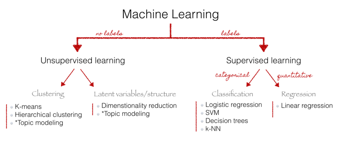
7.3.14 Analysis: Unsupervised text classification

Source: (Christine Doig 2015)

7.3.15 Analysis: Topic Models

Aim:

discovering the hidden (i.e, latent) topics within the documents and assigning each of the topics to the documents
topic modeling: entirely unsupervised classification
- \(\rightarrow\) no prior knowledge of your corpus or possible latent topics is needed (however some knowledge might help you validate your model later on)
Researcher only needs to specify number of topics (not as intuitive as it sounds!)

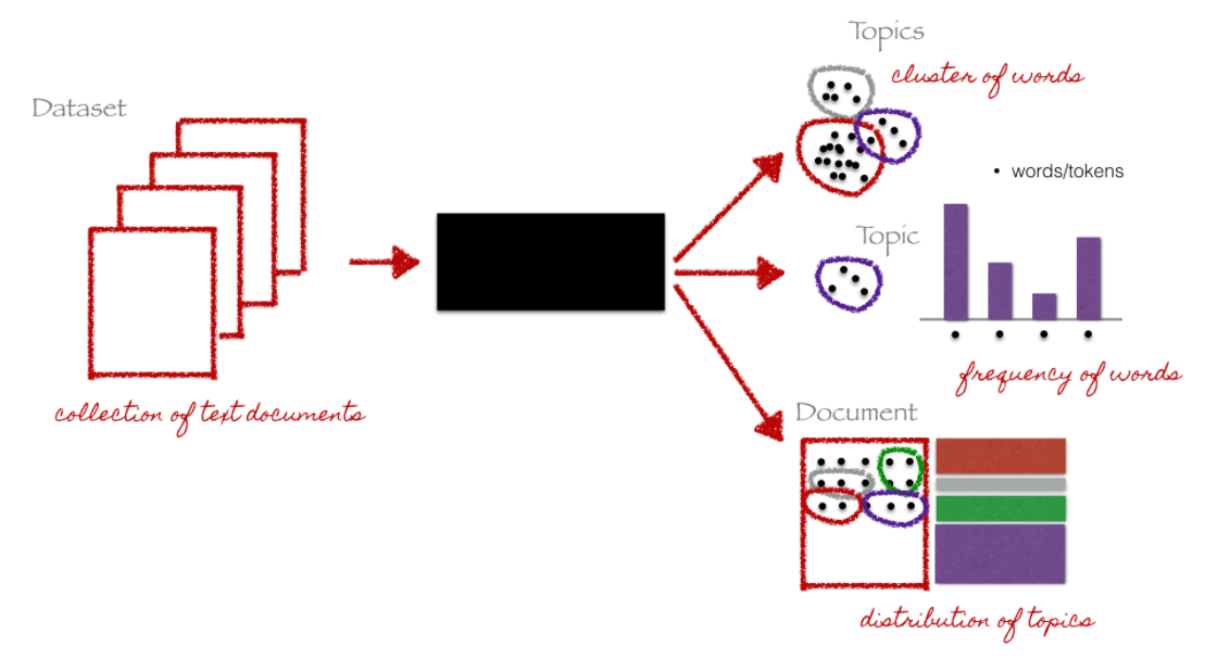
Source: (Christine Doig 2015)

7.3.16 Analysis: Latent Dirichlet Allocation (1)

one of the most popular topic model algorithms
developed by a team of computer linguists (David Blei, Andrew Ng und Michael Jordan, original paper)
two assumptions:
- each document is a mixture over latent topics
  - For example, in a two-topic model we could say “Document 1 is 90% topic A and 10% topic B, while Document 2 is 30% topic A and 70% topic B.”
- each topic is a mixture of words (with possible overlap)

Below, have a look at one examplary output of a LDA, provided by Blei et al. in their paper. The corpus here consists of news articles, while the graph below shows one examplary document. By calculating a LDA the authors find 4 topics (which they labelled Arts, Budgets, Children and Education). The upper part of the graph displays those 4 topics with their respective most common words. Consider, that each column here only shows some of the top words.

Small note: For instance, the term “receive” is colored in green here (e.g. it is assigned to the “Budgets”-topic), whereas “receive” in this graph is only visible as a top word for the “Education”-topic. This is a somewhat unfortunate aspect of this graph, however it is a good demonstration of the probabilistic nature of the algorithm behind LDA models \(\rightarrow\) LDA works with (two) probabilities (more information on the next slide) and in this case, due to the context of this certain document, the algorithm decided to assign the term “receive” to topic 2 and not to topic 4 (if we assume that “receive” also appears at some place in the most common words for the “Budgets”-topic).

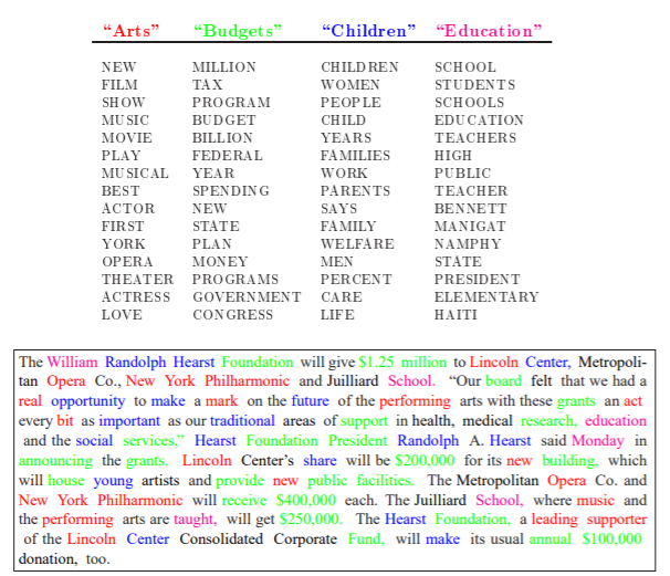
Source: (Blei, Ng, Jordan (2003))

7.3.17 Analysis: Latent Dirichlet Allocation (2)

specify number of topics (k)
each word (w) in each document (d) is randomly assigned to one topic (assignment involves a Dirichlet distribution)
these topic assignments for each word w are then updated in an iterative fashion (Gibbs Sampler)

namely: again, for each word in each document two probabilities are repeatedly calculated:
- 1. “document”-level: proportion of words in document d belonging to a certain topic t (beta) (relative importance of topics in documents)
- 1. “word”-level: proportion of words being assigned to a certain topic t in all other documents (gamma) (relative importance of words in topics)
each word is reassigned to a new topic which is chosen as the probability of p = beta x gamma (overall probability that a certian topic generated the respective word w, put differently: overall probability that that w belongs to topic 1, 2, 3 or 4 (if k was set to 4)

Assignment stops after user-specified threshold, or when iterations begin to have little impact on the probabilities assigned to words in the corpus

7.3.18 Analysis: Structural Topic Models

Structural Topic Models (STM) employs main ideas of LDA but adds a couple more features on top (for an detailed explanation of differences between LDA and STM, read here
- e.g., STM recognizes if topics might be related to one another (e.g., if document 1 contains topic A it might be very likely that it also contains topic B, but not topic C - Correlated Topic Model)
especially useful for social scientists who are interested in modeling effects of covariates (e.g., year, author, sociodemographics, time as a covariate, source)
generally, by allowing to include such metadata STM exceeds a simple bag-of-words approach