6.20 Lab: Predicting recidvism (Classification)
Our lab is based on Lee, Du, and Guerzhoy (2020) and on James et al. (2013 Chap. 4.6.2) with various modifications I made. We will be using the dataset at LINK that is described by Angwin et al. (2016). It’s data based on the COMPAS risk assessment tools (RAT). RATs are increasingly being used to assess a criminal defendant’s probability of re-offending. While COMPAS seemingly uses a larger number of features/variables for the prediction, Dressel and Farid (2018) showed that a model that includes only a defendant’s sex, age, and number of priors (prior offences) can be used to arrive at predictions of equivalent quality.
We first import the data into R:
library(tidyverse)
set.seed(0)
# data <- read.csv("https://github.com/propublica/compas-analysis/raw/master/compas-scores-two-years.csv")
# write_csv(data, "compas-scores-two-years.csv")
data <- read_csv("compas-scores-two-years.csv")
Then we create a factor version of is_recid that we label (so that we can look up what is what aftewards). We also order our variabels differently.
data$is_recid_factor <- factor(data$is_recid,
                        levels = c(0,1),
                        labels = c("no", "yes"))
data <- data %>% select(id, name, compas_screening_date, is_recid,
                        is_recid_factor, age, priors_count, everything())
6.20.1 Inspecting the dataset
First we should make sure to really explore/unterstand our data. How many observations are there? How many different variables (features) are there? What is the scale of the outcome? What are the averages etc.? What kind of units are in your dataset?
## [1] 7214## [1] 54## tibble [7,214 x 54] (S3: tbl_df/tbl/data.frame)
## $ id : num [1:7214] 1 3 4 5 6 7 8 9 10 13 ...
## $ name : chr [1:7214] "miguel hernandez" "kevon dixon" "ed philo" "marcu brown" ...
## $ compas_screening_date : Date[1:7214], format: "2013-08-14" "2013-01-27" ...
## $ is_recid : num [1:7214] 0 1 1 0 0 0 1 0 0 1 ...
## $ is_recid_factor : Factor w/ 2 levels "no","yes": 1 2 2 1 1 1 2 1 1 2 ...
## $ age : num [1:7214] 69 34 24 23 43 44 41 43 39 21 ...
## $ priors_count : num [1:7214] 0 0 4 1 2 0 14 3 0 1 ...
## $ first : chr [1:7214] "miguel" "kevon" "ed" "marcu" ...
## $ last : chr [1:7214] "hernandez" "dixon" "philo" "brown" ...
## $ sex : chr [1:7214] "Male" "Male" "Male" "Male" ...
## $ dob : Date[1:7214], format: "1947-04-18" "1982-01-22" ...
## $ age_cat : chr [1:7214] "Greater than 45" "25 - 45" "Less than 25" "Less than 25" ...
## $ race : chr [1:7214] "Other" "African-American" "African-American" "African-American" ...
## $ juv_fel_count : num [1:7214] 0 0 0 0 0 0 0 0 0 0 ...
## $ decile_score : num [1:7214] 1 3 4 8 1 1 6 4 1 3 ...
## $ juv_misd_count : num [1:7214] 0 0 0 1 0 0 0 0 0 0 ...
## $ juv_other_count : num [1:7214] 0 0 1 0 0 0 0 0 0 0 ...
## $ days_b_screening_arrest: num [1:7214] -1 -1 -1 NA NA 0 -1 -1 -1 428 ...
## $ c_jail_in : POSIXct[1:7214], format: "2013-08-13 06:03:42" "2013-01-26 03:45:27" ...
## $ c_jail_out : POSIXct[1:7214], format: "2013-08-14 05:41:20" "2013-02-05 05:36:53" ...
## $ c_case_number : chr [1:7214] "13011352CF10A" "13001275CF10A" "13005330CF10A" "13000570CF10A" ...
## $ c_offense_date : Date[1:7214], format: "2013-08-13" "2013-01-26" ...
## $ c_arrest_date : Date[1:7214], format: NA NA ...
## $ c_days_from_compas : num [1:7214] 1 1 1 1 76 0 1 1 1 308 ...
## $ c_charge_degree : chr [1:7214] "F" "F" "F" "F" ...
## $ c_charge_desc : chr [1:7214] "Aggravated Assault w/Firearm" "Felony Battery w/Prior Convict" "Possession of Cocaine" "Possession of Cannabis" ...
## $ r_case_number : chr [1:7214] NA "13009779CF10A" "13011511MM10A" NA ...
## $ r_charge_degree : chr [1:7214] NA "(F3)" "(M1)" NA ...
## $ r_days_from_arrest : num [1:7214] NA NA 0 NA NA NA 0 NA NA 0 ...
## $ r_offense_date : Date[1:7214], format: NA "2013-07-05" ...
## $ r_charge_desc : chr [1:7214] NA "Felony Battery (Dom Strang)" "Driving Under The Influence" NA ...
## $ r_jail_in : Date[1:7214], format: NA NA ...
## $ r_jail_out : Date[1:7214], format: NA NA ...
## $ violent_recid : logi [1:7214] NA NA NA NA NA NA ...
## $ is_violent_recid : num [1:7214] 0 1 0 0 0 0 0 0 0 1 ...
## $ vr_case_number : chr [1:7214] NA "13009779CF10A" NA NA ...
## $ vr_charge_degree : chr [1:7214] NA "(F3)" NA NA ...
## $ vr_offense_date : Date[1:7214], format: NA "2013-07-05" ...
## $ vr_charge_desc : chr [1:7214] NA "Felony Battery (Dom Strang)" NA NA ...
## $ type_of_assessment : chr [1:7214] "Risk of Recidivism" "Risk of Recidivism" "Risk of Recidivism" "Risk of Recidivism" ...
## $ decile_score.1 : num [1:7214] 1 3 4 8 1 1 6 4 1 3 ...
## $ score_text : chr [1:7214] "Low" "Low" "Low" "High" ...
## $ screening_date : Date[1:7214], format: "2013-08-14" "2013-01-27" ...
## $ v_type_of_assessment : chr [1:7214] "Risk of Violence" "Risk of Violence" "Risk of Violence" "Risk of Violence" ...
## $ v_decile_score : num [1:7214] 1 1 3 6 1 1 2 3 1 5 ...
## $ v_score_text : chr [1:7214] "Low" "Low" "Low" "Medium" ...
## $ v_screening_date : Date[1:7214], format: "2013-08-14" "2013-01-27" ...
## $ in_custody : Date[1:7214], format: "2014-07-07" "2013-01-26" ...
## $ out_custody : Date[1:7214], format: "2014-07-14" "2013-02-05" ...
## $ priors_count.1 : num [1:7214] 0 0 4 1 2 0 14 3 0 1 ...
## $ start : num [1:7214] 0 9 0 0 0 1 5 0 2 0 ...
## $ end : num [1:7214] 327 159 63 1174 1102 ...
## $ event : num [1:7214] 0 1 0 0 0 0 1 0 0 1 ...
## $ two_year_recid : num [1:7214] 0 1 1 0 0 0 1 0 0 1 ...| Unique (#) | Missing (%) | Mean | SD | Min | Median | Max | ||
|---|---|---|---|---|---|---|---|---|
| id | 7214 | 0 | 5501.3 | 3175.7 | 1.0 | 5509.5 | 11001.0 | |
| is_recid | 2 | 0 | 0.5 | 0.5 | 0.0 | 0.0 | 1.0 | |
| age | 65 | 0 | 34.8 | 11.9 | 18.0 | 31.0 | 96.0 | |
| priors_count | 37 | 0 | 3.5 | 4.9 | 0.0 | 2.0 | 38.0 | |
| juv_fel_count | 11 | 0 | 0.1 | 0.5 | 0.0 | 0.0 | 20.0 | |
| decile_score | 10 | 0 | 4.5 | 2.9 | 1.0 | 4.0 | 10.0 | |
| juv_misd_count | 10 | 0 | 0.1 | 0.5 | 0.0 | 0.0 | 13.0 | |
| juv_other_count | 10 | 0 | 0.1 | 0.5 | 0.0 | 0.0 | 17.0 | |
| days_b_screening_arrest | 424 | 4 | 3.3 | 75.8 | -414.0 | -1.0 | 1057.0 | |
| c_days_from_compas | 500 | 0 | 57.7 | 329.7 | 0.0 | 1.0 | 9485.0 | |
| r_days_from_arrest | 202 | 68 | 20.3 | 74.9 | -1.0 | 0.0 | 993.0 | |
| is_violent_recid | 2 | 0 | 0.1 | 0.3 | 0.0 | 0.0 | 1.0 | |
| decile_score.1 | 10 | 0 | 4.5 | 2.9 | 1.0 | 4.0 | 10.0 | |
| v_decile_score | 10 | 0 | 3.7 | 2.5 | 1.0 | 3.0 | 10.0 | |
| priors_count.1 | 37 | 0 | 3.5 | 4.9 | 0.0 | 2.0 | 38.0 | |
| start | 237 | 0 | 11.5 | 47.0 | 0.0 | 0.0 | 937.0 | |
| end | 1115 | 0 | 553.4 | 399.0 | 0.0 | 530.5 | 1186.0 | |
| event | 2 | 0 | 0.4 | 0.5 | 0.0 | 0.0 | 1.0 | |
| two_year_recid | 2 | 0 | 0.5 | 0.5 | 0.0 | 0.0 | 1.0 |
| N | % | ||
|---|---|---|---|
| is_recid_factor | no | 3743 | 51.9 |
| yes | 3471 | 48.1 | |
| sex | Female | 1395 | 19.3 |
| Male | 5819 | 80.7 | |
| age_cat | 25 - 45 | 4109 | 57.0 |
| Greater than 45 | 1576 | 21.8 | |
| Less than 25 | 1529 | 21.2 | |
| race | African-American | 3696 | 51.2 |
| Asian | 32 | 0.4 | |
| Caucasian | 2454 | 34.0 | |
| Hispanic | 637 | 8.8 | |
| Native American | 18 | 0.2 | |
| Other | 377 | 5.2 | |
| c_charge_degree | F | 4666 | 64.7 |
| M | 2548 | 35.3 | |
| r_charge_degree | (CO3) | 2 | 0.0 |
| (F1) | 51 | 0.7 | |
| (F2) | 168 | 2.3 | |
| (F3) | 892 | 12.4 | |
| (F5) | 1 | 0.0 | |
| (F6) | 3 | 0.0 | |
| (F7) | 7 | 0.1 | |
| (M1) | 1201 | 16.6 | |
| (M2) | 1107 | 15.3 | |
| (MO3) | 39 | 0.5 | |
| vr_charge_degree | (F1) | 38 | 0.5 |
| (F2) | 162 | 2.2 | |
| (F3) | 228 | 3.2 | |
| (F5) | 1 | 0.0 | |
| (F6) | 4 | 0.1 | |
| (F7) | 18 | 0.2 | |
| (M1) | 344 | 4.8 | |
| (M2) | 19 | 0.3 | |
| (MO3) | 5 | 0.1 | |
| Risk of Recidivism | 7214 | 100.0 | |
| score_text | High | 1403 | 19.4 |
| Low | 3897 | 54.0 | |
| Medium | 1914 | 26.5 | |
| Risk of Violence | 7214 | 100.0 | |
| v_score_text | High | 714 | 9.9 |
| Low | 4761 | 66.0 | |
| Medium | 1739 | 24.1 |
| African-American | Asian | Caucasian | Hispanic | Native American | Other |
|---|---|---|---|---|---|
| 3696 | 32 | 2454 | 637 | 18 | 377 |
| no | yes | |
|---|---|---|
| 0 | 3743 | 0 |
| 1 | 0 | 3471 |
| 1 | 2 | 3 | 4 | 5 | 6 | 7 | 8 | 9 | 10 |
|---|---|---|---|---|---|---|---|---|---|
| 1440 | 941 | 747 | 769 | 681 | 641 | 592 | 512 | 508 | 383 |
The variable were named quite well, so that they are often self-explanatory. decile_score is the COMPAS score. is_recid wether someone reoffended (1 = recidividate = reoffend, 0 = NOT). race contains the race. Below we will ignore everyone who wasn’t white or black. age contains age.
6.20.2 Splitting the datasets
As discussed supervised ML requires that we train our ML algorithm with some data which is usually called the training data. In the chunk below we split the dataset be randomly selecting subsets and assigned them to new data objects. Here we split into training data and test data. We use the latter to calculate the test error rate (splitting the original data into two datasets is called “validation set approach” (James et al. 2013, Ch. 5.1.1) (see the next slides for cross-validation).
6.20.3 Comparing the scores of black and white defendants
Below we visualize the COMPAS scores for white and black defendants. We first explore whether white and black defendants get the same COMPAS scores.
Q: What do you see?
data.bw <- data.train %>% filter(race %in% c("African-American", "Caucasian"))

ggplot(data.bw, mapping = aes(x = decile_score)) +
  geom_histogram(bins = 10, mapping = aes(y = ..density..)) +
  scale_x_continuous(breaks = c(1:10)) +
  facet_wrap(~race)  +
  xlab("Decile score") +
  theme_light()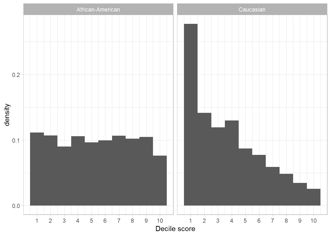
For African-American defendants, the distribution of the scores is approximately uniform. For Caucasian defendants, many more get low scores than high scores as indicated by the right-skewed distribution for Caucasian.
6.20.4 Building a predictiv model
Dressel and Farid (2018) suggest that the COMPAS prediction (which apparently is based on 137 features) can be achieved with a simple linear classifier with only two features. Below we will try to replicate those results. Let’s fit the model now using our training data data.train:
fit <- glm(is_recid ~ age + priors_count,
           family = binomial,
           data = data.train)
#fit$coefficients
summary(fit)
##
## Call:
## glm(formula = is_recid ~ age + priors_count, family = binomial,
## data = data.train)
##
## Deviance Residuals:
## Min 1Q Median 3Q Max
## -3.1354 -1.0623 -0.5582 1.0883 2.5828
##
## Coefficients:
## Estimate Std. Error z value Pr(>|z|)
## (Intercept) 1.078730 0.098085 11.00 <2e-16 ***
## age -0.049021 0.002879 -17.03 <2e-16 ***
## priors_count 0.164027 0.008276 19.82 <2e-16 ***
## ---
## Signif. codes: 0 '***' 0.001 '**' 0.01 '*' 0.05 '.' 0.1 ' ' 1
##
## (Dispersion parameter for binomial family taken to be 1)
##
## Null deviance: 6925.8 on 4999 degrees of freedom
## Residual deviance: 6184.4 on 4997 degrees of freedom
## AIC: 6190.4
##
## Number of Fisher Scoring iterations: 4An increase of 1 in the number of priors is associated with an increase of 0.17 in the log-odds of recidivism, all other things being equal.
An increase in age by one year corresponds to a decrease of 0.05 in the log-odds of recidivism.
(If we’re being a bit silly and decide to extrapolate) according to the model, a newborn with no priors would have a probability of \(\sigma(1.04) = 0.74\) of being re-arrested.
6.20.5 Predicting values
If no data set is supplied predict() computes probabilities for all units in data.train, i.e., the whole dataset (and all individuals) that we used to fit the model (see below). The probability is computed for each individual in our dataset, hence, we get a vector of the length of our dataset. And we can add those predicted probablity to the dataset (then we can check different individuals).
data.train$probs <- predict(fit, type="response") # predict values for everyone and add to data
summary(data.train$probs)| Min. | 1st Qu. | Median | Mean | 3rd Qu. | Max. |
|---|---|---|---|---|---|
| 0.0355982 | 0.3602424 | 0.4878152 | 0.4832 | 0.5813522 | 0.9949583 |
We know that these values correspond to the probability of the recidivating/reoffending (rather than not), because the underlying dummy variable is 1 for reoffending (see use of contrasts() function in James et al. (2013, 158)).
We can also make predictions for particular hypothetical values of our explanatory variables/features:
data_predict = data.frame(age = c(30, 30, 50),
                 priors_count = c(2, 4, 2))
data_predict$Pr <- predict(fit, newdata = data_predict, type = "response")
data_predict| age | priors_count | Pr |
|---|---|---|
| 30 | 2 | 0.4840455 |
| 30 | 4 | 0.5656722 |
| 50 | 2 | 0.2603297 |
We observe an increase of about 8% in the probability when changing the priors_count (number of prior offences) variable from 2 to 4 (keeping age at 30).
6.20.6 Training error rate
The training error rate is the error rate we make using our model in in the training data.
Let’s use our predicted probabilities and we decide that we use a threshold of > 0.5 (of the probability) to classify people as (future) recidivators. Then we can create a second variable classified that contains our model-based classification \(\hat{y}_{i}\) and compare it to the real outcome values \(y_{i}\) that are stored in the variable is_recid.
Q: How would you interpret this table?
data.train <- data.train %>%
              mutate(classified =
                       if_else(probs >= 0.5, 1, 0))
# Table y against predicted y
table(data.train$is_recid,
data.train$classified)| 0 | 1 | |
|---|---|---|
| 0 | 1817 | 767 |
| 1 | 832 | 1584 |
Yes, the diagonal elements of the confusion matrix indicate correct predictions, while the off-diagonals represent incorrect predictions. Subsequently, we can calculate how many errors we made and the training error rate (see Assessing Model Accuracy):
## [1] 1599- Q: How could we calculate the number of errors using the cross table above?
# Training error rate
# same as: sum(data.train$is_recid!=data.train$classified)/nrow(data.train)
mean(data.train$is_recid!=data.train$classified) # Error rate
## [1] 0.3198## [1] 0.6802## [1] 0.6802We can see that 0.32 of the individuals have been classified wrongly by our classifier. 0.68 have been classified correctly.
Q: Do you think this is high? What could be a benchark?
6.20.7 Test error rate
The test error rate is the error rate we make using our model in in the test data.
We did not calculate the test error rate here, so let’s see how our model would perform in the test data data.test that we held out. This error rate should be more realistic because we are interested in our model’s performance not on the data that we used to fit the model, but rather on individuals in the future (hence, individuals the model hasn’t seen yet) (cf. James et al. 2013, 158). So we fit the model (again) on our training data, however, we now use to predict recidvism in the test data.
Above we already created the test dataset data.test.
# Fit the model based on the training data (again)
fit <- glm(is_recid ~ age + priors_count, family = binomial, data = data.train)

# Use model parameters to classify (predict) using the test dataset
# and add to dataset
data.test$probs <- predict(fit, data.test ,type="response")
Here we train and test (classification) our model on two different datasets data.train and data.test. Classification was now performed for the test dataset.
Then we add the classification variable again and calculate our error rates but now for the test data:
# Add classification variable
data.test <- data.test %>%
              mutate(classified =
                       if_else(probs >= 0.5, 1, 0))
mean(data.test$is_recid!=data.test$classified) # Error rate
## [1] 0.317## [1] 0.683We can see that the rates for the test data are very similar to those we obtained from our model for the training data.
6.20.8 Comparison to COMPAS score
So far we haven’t compared our predictions to the predictions made by compass. To start we create a variable classified_COMPAS in data.train that contains the predictions using the COMPAS score decile_score and a cutoff of 5 (= 0.5). Then we table the COMPAS classification against the real recidivsm variable.
data.train <- data.train %>%
              mutate(classified_COMPAS =
                    if_else(decile_score >= 5, 1, 0))
table(data.train$is_recid,
data.train$classified_COMPAS)| 0 | 1 | |
|---|---|---|
| 0 | 1776 | 808 |
| 1 | 939 | 1477 |
To calculate (and compare) the error rate for both the COMPAS classifier and our classifier we can use the following code:
## [1] 0.6506## [1] 0.6802## [1] 0.3494## [1] 0.3198In the training data our classifier seems to work even better than the COMPAS classifier.
In a next step we would compare the accuracy of the two classifiers in the test data (we leave that for now…).
6.20.9 Model comparisons
Normally, we would compare the predictive power of our model to other models.
First, we might try to built a better logistic model. For instance, we could add predictors to see whether the error rate in the predictions decreases (for both the training and the test data). As a very simple illustration we estimate another model fit_new below that only includes one predictor namely age:
# Fit the model based on the training data (again)
# this time only age!
fit_new <- glm(is_recid ~ age,
               family = binomial, data = data.train)

# Add new predicted probs to data
data.train$probs_new <- predict(fit_new, type="response") # predict values for everyone and add to data

# Add new classifications to data
data.train <- data.train %>%
              mutate(classified_new =
                       if_else(probs_new >= 0.5, 1, 0))

# Compare the two error rates agains each other

# Old model (is_recid ~ age + priors_count)
sum(data.train$is_recid!=data.train$classified) # number of errors
## [1] 1599## [1] 0.3198## [1] 2067## [1] 0.4134Q: Does the new model (that includes only age as a predictor) fare worse or better?
Second, we would explore whether other classification methods (models) fare better in terms of model accuracy. To do so we would predict/classify using these other methods. Subsequently, we would compare the error rates.
References
Angwin, Julia, Jeff Larson, Lauren Kirchner, and Surya Mattu. 2016. “Machine Bias.” https://www.propublica.org/article/machine-bias-risk-assessments-in-criminal-sentencing.
Dressel, Julia, and Hany Farid. 2018. “The Accuracy, Fairness, and Limits of Predicting Recidivism.” Sci Adv 4 (1): eaao5580.
James, Gareth, Daniela Witten, Trevor Hastie, and Robert Tibshirani. 2013. An Introduction to Statistical Learning: With Applications in R. Springer Texts in Statistics. Springer.
Lee, Claire S, Jeremy Du, and Michael Guerzhoy. 2020. “Auditing the COMPAS Recidivism Risk Assessment Tool: Predictive Modelling and Algorithmic Fairness in CS1.” In Proceedings of the 2020 ACM Conference on Innovation and Technology in Computer Science Education, 535–36. ITiCSE ’20. New York, NY, USA: Association for Computing Machinery.