8.18 Lab: Predicting house prices: a regression example

Based on Chollet and Allaire (2018 Ch. 3.6) who provide examples for binary, categorical and continuous outcomes.

In the lab below we have a quantitative outcome that we’ll try to predict namely house prices. In other words, instead of predicting discrete labels (classification) we now predict values on a continuous variable

Q: Is that a classification or a regression problem?
The Boston Housing Price dataset (overview)
- Outcome: Median house prices in suburbs (1970s)
- Unit of analysis: Suburb
- Predictors/explanatory variables/features
  - 13 numerical features, such as per capita crime rate, average number of rooms per dwelling, accessibility to highways etc.
  - Each input feature has a different scale
- Data: 506 observations/suburbs (404 training samples, 102 test samples)

8.18.0.1 Load the dataset

We load the dataset (comes as a list) and create four objects using the %<-% operator that is part of the keras package.

library(keras)
library(tensorflow) # should be preloaded

# Dataset comes as a list
dataset <- dataset_boston_housing()
  # The already splits the dataset into training and test data
  # it creates a list

# The data is stored in a list
# Elements 'train' and 'test' contain 
# predictors/features x and outcome y
names(dataset)

## [1] "train" "test"

names(dataset$train)

## [1] "x" "y"

We convert the data in the list to four matrices train_data, train_targets, test_data andtest_targets that we can use in our functions:

# Convert list to matrices
# train_data, train_targets: Training data (predictors, outcome)
# test_data, test_targets: Test data (predictors, outcome)
c(c(train_data, train_targets), c(test_data, test_targets)) %<-% dataset

Let’s look at the data:

head(train_data)

1.23247	0.0	8.14	0.538	6.142	91.7	3.9769	4	307	21.0	396.90	18.72
0.02177	82.5	2.03	0.415	7.610	15.7	6.2700	2	348	14.7	395.38	3.11
4.89822	0.0	18.10	0.631	4.970	100.0	1.3325	24	666	20.2	375.52	3.26
0.03961	0.0	5.19	0.515	6.037	34.5	5.9853	5	224	20.2	396.90	8.01
3.69311	0.0	18.10	0.713	6.376	88.4	2.5671	24	666	20.2	391.43	14.65
0.28392	0.0	7.38	0.493	5.708	74.3	4.7211	5	287	19.6	391.13	11.74

head(test_data)

18.08460	18.10	0	0.679	6.434	100.0	1.8347	24	666	20.2	27.25	29.05
0.12329	10.01	0	0.547	5.913	92.9	2.3534	6	432	17.8	394.95	16.21
0.05497	5.19	0	0.515	5.985	45.4	4.8122	5	224	20.2	396.90	9.74
1.27346	19.58	1	0.605	6.250	92.6	1.7984	5	403	14.7	338.92	5.50
0.07151	4.49	0	0.449	6.121	56.8	3.7476	3	247	18.5	395.15	8.44
0.27957	9.69	0	0.585	5.926	42.6	2.3817	6	391	19.2	396.90	13.59

We have 404 training samples and 102 test samples, each with 13 numerical features, such as per capita crime rate, average number of rooms per dwelling, accessibility to highways, and so on.

Below we also inspect our outcome that we want to predict:

str(train_targets)

##  num [1:404(1d)] 15.2 42.3 50 21.1 17.7 18.5 11.3 15.6 15.6 14.4 ...

summary(train_targets)

Min.	1st Qu.	Median	Mean	3rd Qu.	Max.
5	16.675	20.75	22.39505	24.8	50

str(test_targets)

##  num [1:102(1d)] 7.2 18.8 19 27 22.2 24.5 31.2 22.9 20.5 23.2 ...

The targets (the outcome we want to predict) are the median values of owner-occupied homes, in thousands of dollars. The prices are typically between 10,000$ and 50,000$ (prices are not adjusted for inflation, 1970s).

8.18.0.2 Preparing the input data

Learning for a neural network is more difficult when the input data has wildly different ranges (the network should be able to adapt but it takes longer)
Chollet and Allaire (2018) recommend the “widespread best practice” of feature-wise normalization
- for each feature in the input data (a column in the input data matrix), you subtract the mean of the feature and divide by the standard deviation, so that the feature is centered around 0 and has a unit standard deviation
- We use the scale() for that

# Calculate the mean and standard deviation 
# for each column of training data

mean <- apply(train_data, 2, mean)                               
std <- apply(train_data, 2, sd)

# Scale the training and test data using the mean(s) and 
# standard deviation(s) from the training data
train_data <- scale(train_data, center = mean, scale = std)        
test_data <- scale(test_data, center = mean, scale = std)

Important: The quantities used for normalizing the test data are computed using the training data.

!! Never use in your workflow any quantity computed on the test data, even for something as simple as data normalization !!

8.18.0.3 Building your network

We use a a small network with two hidden layers, each with 64 units, because of the small number of samples (small size of data)
General rule: The less training data we have, the worse overfitting will be, and using a small network is one way to mitigate overfitting.

Because we will need to instantiate the same model multiple times, we use a function to construct it.

# Model definition (as a function)
build_model <- function() {
  # Define network architecture
  model <- keras_model_sequential() %>%
    layer_dense(units = 64, activation = "relu",
                input_shape = dim(train_data)[[2]]) %>%
    layer_dense(units = 64, activation = "relu") %>%
    layer_dense(units = 1) # Ends with single unit
  # Set loss function, optimizer and metric
  model %>% compile(
    optimizer = "rmsprop",
    loss = "mse", # Mean squared error loss function
    metrics = c("mae") # mean absolute error (MAE)
  )
}
# MSE = mean squared error = square of the difference between 
# the predictions and the targets

The network ends with a single unit and no activation (it will be a linear layer)
- This is a typical setup for scalar regression where we are trying to predict a single continuous value
- Here: Last layer is purely linear so that network is free to learn to predict values in any range
Applying another activation function would constrain the range the output can take
- e.g., applying sigmoid activation function to the last layer, the network could only learn to predict values between 0 and 1
Loss function
- Mean squared error: the square of the difference between the predictions and the targets (standard loss function for regression problems)
Metric for monitoring: mean absolute error (MAE)
- Absolute value of the difference between the predictions and the targets
- e.g., MAE of 0.5 here would mean predictions are off by 500$ on average

8.18.0.4 Validating our approach using K-fold validation

Our dataset is relatively small (remember our discussion of bias/size of training and validation data!)
Best practice: Use K-fold cross-validation (see Figure 8.8)
- Split available data into K partitions (typically K = 4 or 5)
  - Create K identical models and train each one on $K-1$ partitions while evaluating on remaining partition
  - Validation score for model used is then the average of the $K$ validation scores obtained

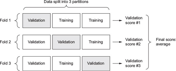
Figure 8.8: The loss score is used as a feedback signal to adjust the weights (Chollet & Allaire, 2018, Fig. 3.9)

Below the code for this procedure:

# K-fold validation
k <- 4 # Number of partitions
indices <- sample(1:nrow(train_data)) # Create indicee used for K folds

# Create folds (4 numbers)
folds <- cut(indices, breaks = k, labels = FALSE) 

num_epochs <- 50
all_scores <- c() # Object to store results

# Loop over K (= folds)
for (i in 1:k) {
  cat("processing fold #", i, "\n")

# Prepare the validation data: data from partition #k
  val_indices <- which(folds == i, arr.ind = TRUE)                     
  val_data <- train_data[val_indices,]
  val_targets <- train_targets[val_indices]

# Prepare the training data: data from all other partitions
  partial_train_data <- train_data[-val_indices,]                      
  partial_train_targets <- train_targets[-val_indices]

# Builds the Keras model (already compiled)
  model <- build_model()         

# Train the model (in silent mode, verbose = 0)
  model %>% fit(partial_train_data, partial_train_targets,             
                epochs = num_epochs, batch_size = 1, verbose = 0)

# Evaluate model on the validation data
  results <- model %>% evaluate(val_data, val_targets, verbose = 0)    
  all_scores <- c(all_scores, results["mae"])
}

## processing fold # 1 
## processing fold # 2 
## processing fold # 3 
## processing fold # 4

Running this with 50 epochs yields the following results:

all_scores

##      mae      mae      mae      mae 
## 2.107852 2.255946 2.670365 2.599349

mean(all_scores)

## [1] 2.408378

mean(all_scores)*1000 # = USD

## [1] 2408.378

The different runs do indeed show rather different validation scores
Average 2.41 is a much more reliable metric than any single score - that’s the entire point of K-fold cross-validation
We are off by 2410$ on average
- This is significant considering that the prices range from 10000$ to 50000$ (variable is in thousands, i.e., divided by 1000)

Below we train the network longer and increase the number of epochs to 200
We also save the per-epoch validation score log to evaluate how it develops across epochs (check how well the model does at each epoch!)

# Below we save the validation logs at each fold

num_epochs <- 200
all_mae_histories <- NULL

# Loop over K (= folds)
for (i in 1:k) {
  cat("processing fold #", i, "\n")

# Prepares the validation data: data from partition #k
  val_indices <- which(folds == i, arr.ind = TRUE)              
  val_data <- train_data[val_indices,]
  val_targets <- train_targets[val_indices]

# Prepares the training data: data from all other partitions
  partial_train_data <- train_data[-val_indices,]               
  partial_train_targets <- train_targets[-val_indices]

# Builds the Keras model (already compiled)
  model <- build_model()  

# Trains the model (in silent mode, verbose=0)
  history <- model %>% fit(                                     
    partial_train_data, partial_train_targets,
    validation_data = list(val_data, val_targets),
    epochs = num_epochs, batch_size = 1, verbose = 0
  )

# Store metrics (validation score)
  mae_history <- history$metrics$val_mae
  all_mae_histories <- rbind(all_mae_histories, mae_history)
}

## processing fold # 1 
## processing fold # 2 
## processing fold # 3 
## processing fold # 4

Then we compute the average of the per-epoch MAE scores for all folds:

# Building the history of successive mean K-fold validation scores
average_mae_history <- data.frame(
  epoch = seq(1:ncol(all_mae_histories)),
  validation_mae = apply(all_mae_histories, 2, mean)
)

Let’s plot this:

# Figure: Validation MAE by epoch
# Plotting validation scores ()
library(ggplot2)
ggplot(average_mae_history, aes(x = epoch, y = validation_mae)) + geom_line()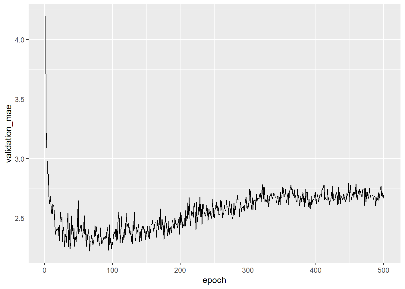

Below we use geom_smooth() to get a better grasp of how the mean absolute error develops across epochs

# Validation MAE by epoch: smoothed
# Plotting validation scores with geom_smooth()
ggplot(average_mae_history, aes(x = epoch, y = validation_mae)) + geom_smooth()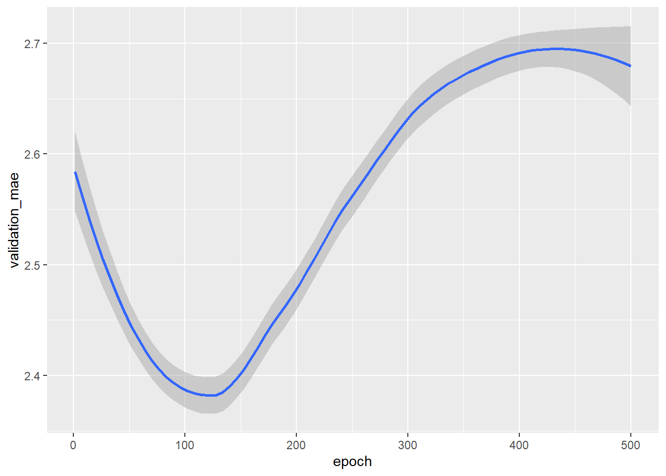

The MAE stops improving significantly after 125 epochs
- After 125 epochs overfitting increases

In other words after 125 the algorithm adapts so strongly to the training data that the predictions for the test data become words again.

8.18.0.5 Confronting the model with test data

Generally, we would tune our model in different ways, e.g., in addition to the number of epochs we could adjust the size of the hidden layers, the number of predictors/features etc.

Then we would train a final production model on all of the training data, with the best parameters, and then look at its performance on the test data.

# Training the final model
model <- build_model()

# Trains the model on the entirety of the data
model %>% fit(train_data, train_targets,                    
          epochs = 80, batch_size = 16, verbose = 0)

# Evaluates the model on the test data
result <- model %>% evaluate(test_data, test_targets)

Here’s the final result for the mean absolute error:

round(result["mae"], 2)

##  mae 
## 3.08

Our model is off by about 2870 $ when trying to predict the test data.

8.18.0.6 Wrapping up & takeaways

Above we discussed a DL example for a regression problem. An example for a classical ML analogue with the same data can be found in Chapter 3.6 in James et al. (2013). For DL examples for binary and categorical outcomes see the Chapter 3.4 and 3.5 in Chollet and Allaire (2018).

Loss functions
- Regression uses different loss functions than classification (e.g., error rate)
- Mean squared error (MSE) is a loss function commonly used for regression
Evaluation metrics
- Differ for regression and classification
- Common regression metric is mean absolute error (MAE)
Preprocessing
- When features in input data have values in different ranges, each feature should be scaled independently as a preprocessing step
Small datasets
- K-fold validation is a great way to reliably evaluate a model
- Preferable to use a small network with few hidden layers (typically only one or two), in order to avoid severe overfitting

8.18.0.7 Summary

ML (or DL) models can be built for different outcome: binary variables (classification), categorical variables (classification), continuous variables (regression)
Preprocessing: When the data has features (explanatory vars) with different ranges, we would scale each feature as part of the preprocessing
Overfitting: As training progresses, neural networks eventually begin to overfit and obtain worse resutls for never-before-seen data
If you don’t have much training data, use a small network with only one or two hidden layers, to avoid severe overfitting
Layer number: If data divided into many categories, making the layers to small may cause information bottlenecks
Loss functions: Regression uses different loss functions and different evaluation metrics than classification
Data size: K-fold validation can help reliably evaluate your model when the data is small

References

Chollet, Francois, and J J Allaire. 2018. Deep Learning with R. 1st ed. Manning Publications.

James, Gareth, Daniela Witten, Trevor Hastie, and Robert Tibshirani. 2013. An Introduction to Statistical Learning: With Applications in R. Springer Texts in Statistics. Springer.