7 Tidy data

7.1 Objectives

• Restructure data tabulations with pivot_wider() and pivot_longer()

• using ungroup() to remove the effect of a group_by() function

7.2 Reading

Garrett Grolemund and Hadley Wickham, R for Data Science

• 12. Tidy data, sections 12.1 to 12.3

• 6. Workflow: scripts

Karl Broman & Kara Woo, “Data Organization in Spreadsheets”(Broman and Woo 2017)

Julie Lowndes and Allison Horst, “Tidy Data for Efficiency, Reproducibility, and Collaboration”)(Lowndes and Horst 2020)

• {tidyr} reference at tidyverse.org

7.3 Transform Data 3: changing the layout

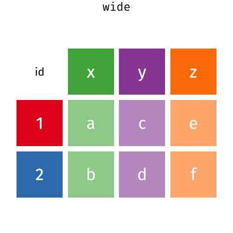
7.3.1 Tidy and untidy data

In the dataframes we have used so far, the data is in a format that adheres to the rules of tidy data, where

• each column is a variable
• each row is an observation
• each value has its own cell

This is called a “long” data format. But, we notice that each column represents a different variable. In the “longest” data format there would only be three columns, one for the id variable, one for the observed variable, and one for the observed value (of that variable). This data format is quite unsightly and difficult to work with, so you will rarely see it in use.

Alternatively, in a “wide” data format we see modifications to rule 1, where each column no longer represents a single variable. Instead, columns can represent different levels/values of a variable. For instance, in some data you encounter the researchers may have chosen for every survey date to be a different column.

These may sound like dramatically different data layouts, but there are some tools that make transitions between these layouts much simpler than you might think! The gif below shows how these two formats relate to each other, and gives you an idea of how we can use R to shift from one format to the other.

(From the Data Carpentry lesson R for Social Scientists, “Data Wrangling with dplyr and tidyr”—this lesson provides a different example of using {tidyr} to reshape your data.)

The image below shows the relationship between the two versions of the same data:[@AdenBuie_tidyanimated]

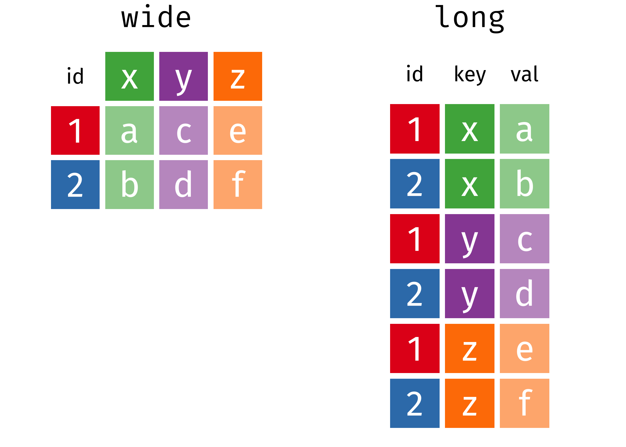
The “wide” form doesn’t adhere to the rules of tidy data, since each row has multiple observations.

Untidy data most often look like this: * Column headers are values, not variable names. * Multiple variables are stored in one column. * Variables are stored in both rows and columns. * Multiple types of observational units are stored in the same table. * A single observational unit is stored in multiple tables.

(Source: John Spencer, “Tidy Data and How to Get It”)

7.3.2 An example

Let’s create a pivot table crosstab using the {mpg} data package of automobile fuel economy.

First, a look at the source table.

mpg

## # A tibble: 234 × 12
##    manufacturer model      displ  year   cyl trans    drv     cty   hwy fl    class mpg_per_cubic_l…
##    <chr>        <chr>      <dbl> <int> <int> <chr>    <chr> <int> <int> <chr> <chr>            <dbl>
##  1 audi         a4           1.8  1999     4 auto(l5) f        18    29 p     comp…            16.1 
##  2 audi         a4           1.8  1999     4 manual(… f        21    29 p     comp…            16.1 
##  3 audi         a4           2    2008     4 manual(… f        20    31 p     comp…            15.5 
##  4 audi         a4           2    2008     4 auto(av) f        21    30 p     comp…            15   
##  5 audi         a4           2.8  1999     6 auto(l5) f        16    26 p     comp…             9.29
##  6 audi         a4           2.8  1999     6 manual(… f        18    26 p     comp…             9.29
##  7 audi         a4           3.1  2008     6 auto(av) f        18    27 p     comp…             8.71
##  8 audi         a4 quattro   1.8  1999     4 manual(… 4        18    26 p     comp…            14.4 
##  9 audi         a4 quattro   1.8  1999     4 auto(l5) 4        16    25 p     comp…            13.9 
## 10 audi         a4 quattro   2    2008     4 manual(… 4        20    28 p     comp…            14   
## # … with 224 more rows

Use group_by and summarise to create a summary table of the average engine displacement:

mpg %>%                                
  group_by(class) %>%                   
  summarise(displ_mean = mean(displ)) 

## # A tibble: 7 × 2
##   class      displ_mean
##   <chr>           <dbl>
## 1 2seater          6.16
## 2 compact          2.33
## 3 midsize          2.92
## 4 minivan          3.39
## 5 pickup           4.42
## 6 subcompact       2.66
## 7 suv              4.46

Now if we do the same with vehicle class and number of cylinders, we end up with a much longer table. Since we are going to restructure this table, it will be assigned to a new object class_by_cyl.

class_by_cyl <- mpg %>%
  group_by(class, cyl) %>%
  summarise(displ_mean = mean(displ)) %>%
  arrange(desc(displ_mean))

class_by_cyl

## # A tibble: 19 × 3
## # Groups:   class [7]
##    class        cyl displ_mean
##    <chr>      <int>      <dbl>
##  1 2seater        8       6.16
##  2 suv            8       5.16
##  3 pickup         8       4.96
##  4 subcompact     8       4.76
##  5 midsize        8       4.75
##  6 pickup         6       3.84
##  7 suv            6       3.75
##  8 minivan        6       3.49
##  9 subcompact     6       3.39
## 10 midsize        6       3.22
## 11 compact        6       2.94
## 12 pickup         4       2.7 
## 13 suv            4       2.55
## 14 compact        5       2.5 
## 15 subcompact     5       2.5 
## 16 minivan        4       2.4 
## 17 midsize        4       2.26
## 18 compact        4       2.07
## 19 subcompact     4       1.93

While this long tabular structure is useful for coding, it’s harder for you and I to compare across both the “class” and “cyl” dimensions. This is a situation where a wide structure is desirable.

7.3.3 pivot_wider()

Let’s take the class_by_cyl table and arrange it so that there is a separate variable for each number of cylinders. Instead of a single “cyl” column, there will be multiple columns, one for each category of cylinder count.

You will note that this is NOT a tidy format! But is it one that is human-readable, and is often how data tables are published in reports.

# pivot table (wide)

class_by_cyl_pivot <- class_by_cyl %>%
  pivot_wider(names_from = cyl, values_from = displ_mean)

class_by_cyl_pivot

## # A tibble: 7 × 5
## # Groups:   class [7]
##   class        `8`   `6`   `4`   `5`
##   <chr>      <dbl> <dbl> <dbl> <dbl>
## 1 2seater     6.16 NA    NA     NA  
## 2 suv         5.16  3.75  2.55  NA  
## 3 pickup      4.96  3.84  2.7   NA  
## 4 subcompact  4.76  3.39  1.93   2.5
## 5 midsize     4.75  3.22  2.26  NA  
## 6 minivan    NA     3.49  2.4   NA  
## 7 compact    NA     2.94  2.07   2.5

Note that the table is sorted by the order in which the variables are encountered in the data; “class” is not alphabetical, and the cylinder numbers are also not ordered. Below are two solutions that result in the table variables being sorted.

# sort with `arrange()`
class_by_cyl %>%
  # sort before pivot
  arrange(cyl, class) %>% 
  pivot_wider(names_from = cyl, values_from = displ_mean)

## # A tibble: 7 × 5
## # Groups:   class [7]
##   class        `4`   `5`   `6`   `8`
##   <chr>      <dbl> <dbl> <dbl> <dbl>
## 1 compact     2.07   2.5  2.94 NA   
## 2 midsize     2.26  NA    3.22  4.75
## 3 minivan     2.4   NA    3.49 NA   
## 4 pickup      2.7   NA    3.84  4.96
## 5 subcompact  1.93   2.5  3.39  4.76
## 6 suv         2.55  NA    3.75  5.16
## 7 2seater    NA     NA   NA     6.16

# sort with `names_sort =` argument in `pivot_wider()` function
class_by_cyl %>%
  arrange(cyl, class) %>% 
  # sort within the `pivot_wider()`
  pivot_wider(names_from = cyl, values_from = displ_mean,
              names_sort = TRUE)

## # A tibble: 7 × 5
## # Groups:   class [7]
##   class        `4`   `5`   `6`   `8`
##   <chr>      <dbl> <dbl> <dbl> <dbl>
## 1 compact     2.07   2.5  2.94 NA   
## 2 midsize     2.26  NA    3.22  4.75
## 3 minivan     2.4   NA    3.49 NA   
## 4 pickup      2.7   NA    3.84  4.96
## 5 subcompact  1.93   2.5  3.39  4.76
## 6 suv         2.55  NA    3.75  5.16
## 7 2seater    NA     NA   NA     6.16

7.3.4 pivot_longer()

Now, unpivot it back to the original structure. Note that the names of the new variables “cyl” and “displ_mean” need to be inside quotation marks!

# and back to longer...

displ_class_by_cyl <- class_by_cyl_pivot %>%
  pivot_longer(-class, names_to = "cyl", values_to = "displ_mean")

displ_class_by_cyl

## # A tibble: 28 × 3
## # Groups:   class [7]
##    class   cyl   displ_mean
##    <chr>   <chr>      <dbl>
##  1 2seater 8           6.16
##  2 2seater 6          NA   
##  3 2seater 4          NA   
##  4 2seater 5          NA   
##  5 suv     8           5.16
##  6 suv     6           3.75
##  7 suv     4           2.55
##  8 suv     5          NA   
##  9 pickup  8           4.96
## 10 pickup  6           3.84
## # … with 18 more rows

What do you notice about the structure of the unpivoted table?

The creation of the wider table introduced “NA” values where there was not a “cyl” category to match the “class” of vehicle. In our new long table, those “NA” values have been retained.

7.3.5 spread() and gather()

Note that pivot_wider() and pivot_longer() are relatively new functions, introduced in 2019.

The older {tidyr} functions that do the same thing: spread() and gather(). You may find older articles that use these functions…but the new ones are much better!

For example, spread() to replicate the pivot_wider() function:

class_by_cyl %>%
  spread(cyl, value = displ_mean)

## # A tibble: 7 × 5
## # Groups:   class [7]
##   class        `4`   `5`   `6`   `8`
##   <chr>      <dbl> <dbl> <dbl> <dbl>
## 1 2seater    NA     NA   NA     6.16
## 2 compact     2.07   2.5  2.94 NA   
## 3 midsize     2.26  NA    3.22  4.75
## 4 minivan     2.4   NA    3.49 NA   
## 5 pickup      2.7   NA    3.84  4.96
## 6 subcompact  1.93   2.5  3.39  4.76
## 7 suv         2.55  NA    3.75  5.16

7.3.6 A longer example

First step: review the structure of the mpg data set:

mpg

## # A tibble: 234 × 12
##    manufacturer model      displ  year   cyl trans    drv     cty   hwy fl    class mpg_per_cubic_l…
##    <chr>        <chr>      <dbl> <int> <int> <chr>    <chr> <int> <int> <chr> <chr>            <dbl>
##  1 audi         a4           1.8  1999     4 auto(l5) f        18    29 p     comp…            16.1 
##  2 audi         a4           1.8  1999     4 manual(… f        21    29 p     comp…            16.1 
##  3 audi         a4           2    2008     4 manual(… f        20    31 p     comp…            15.5 
##  4 audi         a4           2    2008     4 auto(av) f        21    30 p     comp…            15   
##  5 audi         a4           2.8  1999     6 auto(l5) f        16    26 p     comp…             9.29
##  6 audi         a4           2.8  1999     6 manual(… f        18    26 p     comp…             9.29
##  7 audi         a4           3.1  2008     6 auto(av) f        18    27 p     comp…             8.71
##  8 audi         a4 quattro   1.8  1999     4 manual(… 4        18    26 p     comp…            14.4 
##  9 audi         a4 quattro   1.8  1999     4 auto(l5) 4        16    25 p     comp…            13.9 
## 10 audi         a4 quattro   2    2008     4 manual(… 4        20    28 p     comp…            14   
## # … with 224 more rows

Run the chunk below to create the displ_class_by_cyl table:

• group the cars by class and cylinder size, and

• show the mean displacement (engine size)

# summary table - class by cylinder
displ_class_by_cyl <- mpg %>%
  group_by(class, cyl) %>%
  summarise(displ_mean = mean(displ)) %>%
  arrange(cyl, class) %>%
  pivot_wider(names_from = cyl, values_from = displ_mean) %>%
  pivot_longer(-class, names_to = "cyl", values_to = "displ_mean")

displ_class_by_cyl

## # A tibble: 28 × 3
## # Groups:   class [7]
##    class   cyl   displ_mean
##    <chr>   <chr>      <dbl>
##  1 compact 4           2.07
##  2 compact 5           2.5 
##  3 compact 6           2.94
##  4 compact 8          NA   
##  5 midsize 4           2.26
##  6 midsize 5          NA   
##  7 midsize 6           3.22
##  8 midsize 8           4.75
##  9 minivan 4           2.4 
## 10 minivan 5          NA   
## # … with 18 more rows

Calculate the mean of displ_mean:

# example
mean(displ_class_by_cyl$displ_mean)

## [1] NA

The “NA” values get in the way of the calculation. If na.rm = TRUE is added to the mean() function, R will calculate the value for us by removing the “NA” values.

# solution
mean(displ_class_by_cyl$displ_mean, na.rm = TRUE)

## [1] 3.438297

An alternative solution: use a filter with !na to remove the records with NA values:

# example
displ_class_by_cyl %>%
  summarise(displ_mean_all = mean(displ_mean))

## # A tibble: 7 × 2
##   class      displ_mean_all
##   <chr>               <dbl>
## 1 2seater             NA   
## 2 compact             NA   
## 3 midsize             NA   
## 4 minivan             NA   
## 5 pickup              NA   
## 6 subcompact           3.14
## 7 suv                 NA

# solution
displ_class_by_cyl %>%
  filter(!is.na(displ_mean)) %>%
  summarise(displ_mean_all = mean(displ_mean))

## # A tibble: 7 × 2
##   class      displ_mean_all
##   <chr>               <dbl>
## 1 2seater              6.16
## 2 compact              2.50
## 3 midsize              3.41
## 4 minivan              2.94
## 5 pickup               3.84
## 6 subcompact           3.14
## 7 suv                  3.82

7.3.7 Summarize with group() and ungroup()

You’ll notice in the example above that when we summarize displ_class_by_cyl it gives the mean values by class, even though we didn’t use any grouping variable.

This is because when we ran the code to create the displ_class_by_cyl table, we grouped by class and cyl. Running the summarise() function is applied, it removes one level of the grouping (in this case, cyl):

# example
displ_class_by_cyl

## # A tibble: 28 × 3
## # Groups:   class [7]
##    class   cyl   displ_mean
##    <chr>   <chr>      <dbl>
##  1 compact 4           2.07
##  2 compact 5           2.5 
##  3 compact 6           2.94
##  4 compact 8          NA   
##  5 midsize 4           2.26
##  6 midsize 5          NA   
##  7 midsize 6           3.22
##  8 midsize 8           4.75
##  9 minivan 4           2.4 
## 10 minivan 5          NA   
## # … with 18 more rows

displ_class_by_cyl %>%
  filter(!is.na(displ_mean)) %>%
  summarise(displ_mean_all = mean(displ_mean))

## # A tibble: 7 × 2
##   class      displ_mean_all
##   <chr>               <dbl>
## 1 2seater              6.16
## 2 compact              2.50
## 3 midsize              3.41
## 4 minivan              2.94
## 5 pickup               3.84
## 6 subcompact           3.14
## 7 suv                  3.82

If you want the mean of all the values, you have to use ungroup() before summarise(), to “peel off” class.

# solution
displ_class_by_cyl %>%
  filter(!is.na(displ_mean)) %>%
  ungroup() %>%
  summarise(displ_mean_all = mean(displ_mean))

## # A tibble: 1 × 1
##   displ_mean_all
##            <dbl>
## 1           3.44

---

7.4 Exercises

7.4.1 Hands-on: Canadian election

This table shows the national-level results of the Federal Election held in Canada on October 10, 2019. This is structure as the table was published by Elections Canada.

## # A tibble: 12 × 3
##    party          category  number
##    <chr>          <chr>      <dbl>
##  1 Liberal        seats        157
##  2 Liberal        votes    5915950
##  3 Conservative   seats        121
##  4 Conservative   votes    6155662
##  5 Bloc Québécois seats         32
##  6 Bloc Québécois votes    1376135
##  7 New Democratic seats         24
##  8 New Democratic votes    2849214
##  9 Green          seats          3
## 10 Green          votes    1162361
## 11 Independent    seats          1
## 12 Independent    votes      75836

What tidy data principles does this table violate?

It violiates Principles #1 & #2

• There are two variables (seats and votes) combined into one column
• There are two rows (seats and rows) for each observation (in this case, party)

Sometimes untidy data can be too long!

Tidy this table’s structure

To tidy the table, we need to pivot_wider()

# solution

CDN_elec_2019 %>%
  pivot_wider(names_from = category, values_from = number)

## # A tibble: 6 × 3
##   party          seats   votes
##   <chr>          <dbl>   <dbl>
## 1 Liberal          157 5915950
## 2 Conservative     121 6155662
## 3 Bloc Québécois    32 1376135
## 4 New Democratic    24 2849214
## 5 Green              3 1162361
## 6 Independent        1   75836

7.4.2 Hands-on: gapminder

When we publish our tables, we might want a structure that violiates the tidy principles—sometimes an untidy table is better for human consumption. The {gapminder} data, in its raw form, is tidy. For this exercise, create a table that shows:

• GDP per capita for
• the countries Canada, United States, and Mexico are the columns, and
• the years after 1980 are the rows

# solution #1
gapminder %>% 
  filter(country %in% c("Canada", "United States", "Mexico") &
           year > 1980) %>%
  select(country, year, gdpPercap) %>% 
  pivot_wider(names_from = country, values_from = gdpPercap)

## # A tibble: 6 × 4
##    year Canada Mexico `United States`
##   <int>  <dbl>  <dbl>           <dbl>
## 1  1982 22899.  9611.          25010.
## 2  1987 26627.  8688.          29884.
## 3  1992 26343.  9472.          32004.
## 4  1997 28955.  9767.          35767.
## 5  2002 33329. 10742.          39097.
## 6  2007 36319. 11978.          42952.

# a similar solution that uses "or" for the countries
# and two separate filter statements
gapminder %>% 
  filter(country == "Canada" | country == "United States" | country == "Mexico") %>% 
  filter(year > 1980) %>%
  select(country, year, gdpPercap) %>% 
  pivot_wider(names_from = country, values_from = gdpPercap)

## # A tibble: 6 × 4
##    year Canada Mexico `United States`
##   <int>  <dbl>  <dbl>           <dbl>
## 1  1982 22899.  9611.          25010.
## 2  1987 26627.  8688.          29884.
## 3  1992 26343.  9472.          32004.
## 4  1997 28955.  9767.          35767.
## 5  2002 33329. 10742.          39097.
## 6  2007 36319. 11978.          42952.

Here’s an alternative approach that avoids the use of the select() function.

Note that by adding year to the pivot_wider() all the variables in the final table are explicitly named in the function, and all the other variables in the source table are dropped.

gapminder %>% 
  filter(country == "Canada" | country == "United States" | country == "Mexico") %>% 
  filter(year > 1980) %>% 
  pivot_wider(id_cols = year, 
              names_from = "country", 
              values_from = "gdpPercap")

## # A tibble: 6 × 4
##    year Canada Mexico `United States`
##   <int>  <dbl>  <dbl>           <dbl>
## 1  1982 22899.  9611.          25010.
## 2  1987 26627.  8688.          29884.
## 3  1992 26343.  9472.          32004.
## 4  1997 28955.  9767.          35767.
## 5  2002 33329. 10742.          39097.
## 6  2007 36319. 11978.          42952.

In this version, the three variables continent, lifeExp, and pop are dropped with the minus sign—the remaining variables are then reshaped.

gapminder %>% 
  filter(country %in% c("Canada", "United States", "Mexico")) %>% 
  filter(year > 1980) %>% 
  pivot_wider(id_cols = c(-continent, -lifeExp, -pop), 
              names_from = "country", 
              values_from = "gdpPercap")

## # A tibble: 6 × 4
##    year Canada Mexico `United States`
##   <int>  <dbl>  <dbl>           <dbl>
## 1  1982 22899.  9611.          25010.
## 2  1987 26627.  8688.          29884.
## 3  1992 26343.  9472.          32004.
## 4  1997 28955.  9767.          35767.
## 5  2002 33329. 10742.          39097.
## 6  2007 36319. 11978.          42952.

(Thanks to the students of BIDA302 spring 2021 for teaching me this one!)

It’s also possible to have multiple columns selected using the id_cols = argument:

# Three countries from three different continents
gapminder %>% 
  filter(country %in% c("Canada", "China", "Croatia")) %>% 
  filter(year > 1980) %>% 
  pivot_wider(id_cols = c(country, continent), 
              names_from = "year", 
              values_from = "gdpPercap")

## # A tibble: 3 × 8
##   country continent `1982` `1987` `1992` `1997` `2002` `2007`
##   <fct>   <fct>      <dbl>  <dbl>  <dbl>  <dbl>  <dbl>  <dbl>
## 1 Canada  Americas  22899. 26627. 26343. 28955. 33329. 36319.
## 2 China   Asia        962.  1379.  1656.  2289.  3119.  4959.
## 3 Croatia Europe    13222. 13823.  8448.  9876. 11628. 14619.

7.4.3 Online exercise

Transform data

• This exercise gives you an opportunity to practice your {dplyr} and {tidyr} skills

---

7.5 Further reading

More about tidy data:

“Tidy Data for Efficiency, Reproducibility, and Collaboration”)

Data Organization in Spreadsheets for Social Scientists: Formatting problems – this DataCarpentry lesson has some good visuals that may help with understanding “names_from” and “names_to” etc.

Reshaping Your Data with tidyr, UC Business Analytics R Programming Guide

• this article uses the old {tidyr} gather() and spread() functions instead of pivot_longer() and pivot_wider(), but it’s got some good material on how to think about how and why data needs to be reshaped.

Julia Lowndes and Allison Horst, Tidy data for efficiency, reproducibility, and collaboration

• in google slide version: “Make friends with tidy data”

Hadley Wickham. “Tidy data”, The Journal of Statistical Software, vol. 59, 2014.

Data organization with spreadsheets – from Data Management Workshop à la CHONe