2 Data profiling and exploration
In this chapter we will explore datasets stored in different data formats, such as csv, json, and xls.
2.1 Aboslute and relative paths
The first step for analyzing data from a data file is to identify the location of the file. If the file is already in the local machine we are working on, we need to identify its path, i.e., its physical location on our local hard drive.
In R, we can get the directory that we are currently located (AKA working director) with the command getwd():
getwd()## [1] "/Users/mkokkodi/Dropbox/teaching/BC/fall2021/isys3350/book"2.1.1 Absolute paths
The printed path starts with a slash /. This slash symbolizes the root directory of our system. Paths that start with / are called absolute paths.
Directoryis a synonym tofolder
Inside the root directory, there are multiple folders. We can see these folders with the help of the command list.files():
list.files("/")## [1] "Applications" "bin" "cores" "dev" "etc"
## [6] "home" "Library" "opt" "private" "sbin"
## [11] "System" "tmp" "Users" "usr" "var"
## [16] "Volumes"As you can see in this example, in the root directory there is a folder Users. Hence, I can access the contents of that folder as follows:
list.files("/Users") ## [1] "bctech" "hatchst" "mkokkodi" "Shared"
I can keep accessing folders within folders by using the same logic:
list.files("/Users/mkokkodi/Dropbox/teaching/BC/fall2021/isys3350/book")## [1] "_book" "_bookdown_files"
## [3] "_main_files" "_main.Rmd"
## [5] "_tmp.Rmd" "A-intro.Rmd"
## [7] "B-data-profiling-and-inputs.Rmd" "book_material"
## [9] "C-API-scraping.Rmd" "D-DDL.Rmd"
## [11] "E-SQL-single-table.Rmd" "F-nba-example.Rmd"
## [13] "figures" "G-SQL-multiple-tables.Rmd"
## [15] "H-SQL-aggregation.Rmd" "I-SQL-subqueries.Rmd"
## [17] "index.Rmd" "J-SQL-advanced_functions.Rmd"
## [19] "K-tidytext.Rmd" "readme.txt"
## [21] "style.css" "Z1-midterm-practice.Rmd"2.1.2 Relative paths
Absolute paths can get very long and convoluted. To simplify, we can often use relative paths. Relative paths do not start with a slash /, but instead, with the name of the directory we want to access that is located within our current working directory. For instance, in my current working directory, there is a folder _book (see previous output). I can check that directory as follows:
list.files("_book/")## [1] "_main_files"
## [2] "404.html"
## [3] "basic-text-analytics.html"
## [4] "case-studey-designing-a-database-for-nba-games.html"
## [5] "case-study-a-database-for-nba-games.html"
## [6] "collecting-structured-and-unstructured-data-from-the-web.html"
## [7] "data-formats.html"
## [8] "data-profiling-and-exploration.html"
## [9] "data-visualization-with-ggplot2.html"
## [10] "dataProfiling.html"
## [11] "figures"
## [12] "index.html"
## [13] "introduction-to-r-and-tidyverse.html"
## [14] "joins.html"
## [15] "libs"
## [16] "midterm-practice-exam.html"
## [17] "search_index.json"
## [18] "sql-advanced-functions.html"
## [19] "sql-aggregating-and-summarizing-results.html"
## [20] "sql-create-and-fill-a-new-database.html"
## [21] "sql-retrieve-data-from-a-single-table.html"
## [22] "sql-retrieve-data-from-multiple-tables.html"
## [23] "sql-subqueries-and-advanced-functions.html"
## [24] "sql-subqueries.html"
## [25] "style.css"From a current working directory we can access its parent directory with two consecutive dots ..:
list.files("..")## [1] "~$llabus-3350.docx" "book" "book_material"
## [4] "create_db_users.ipynb" "data" "figures"
## [7] "isys3350.Rproj" "Midterm key.docx" "README.md"
## [10] "Rmd" "roster_from_grades.csv" "syllabus-3350.docx"
## [13] "syllabus-3350.pdf" "week-1" "week-10"
## [16] "week-11" "week-12" "week-13"
## [19] "week-14" "week-2" "week-3"
## [22] "week-4" "week-5" "week-6"
## [25] "week-9"Hence, we can access the contents of any data folder in that parent directory. For instance, we can access folder data as follows:
list.files("../data/")## [1] "add_records.csv" "alien_income.csv"
## [3] "analytics.csv" "bchashtag.csv"
## [5] "bikes.csv" "colleges.csv"
## [7] "covid.csv" "creditCards.csv"
## [9] "csom.json" "espnTweets"
## [11] "espnTweets.csv" "example.html"
## [13] "example.json" "final_worker.csv"
## [15] "household_power_consumption.txt" "income.csv"
## [17] "nba_practice.csv" "nba.csv"
## [19] "newsSample.csv" "newsTitles.csv"
## [21] "orders.csv" "passengers.csv"
## [23] "predictCustomerSpending.csv" "project_stock.csv"
## [25] "project_viral.csv" "quotes.html"
## [27] "retail.xlsx" "reviewsSample.csv"
## [29] "songs.csv" "stranger_things.csv"
## [31] "trafficAggregated.csv" "tweetsExam.csv"
## [33] "tweetsPracticeExam.csv" "users.csv"
## [35] "wiki.csv" "wikiConcepts.csv"
## [37] "wordcloud.csv" "workerMarket.csv"
## [39] "yahoo.html" "yelp.csv"In your RStudio Cloud system you have saved your current R Markdown file in the
Rmddirectory. Hence your current working directory is theRmdfolder. FromRmd, you can access data files located in thedatafolder by using../data/.
2.2 Different file types
Once we know the location of a data file we can load it into a tibble with the help of various functions that handle different file formats.
2.2.1 Loading CSV files into tibbles
A CSV file is a file with comma-separated values.
Function read_csv of the package readr allows us to load CSV files into tibbles. The package readr is included in the set of tidyverse packages. Recall (see Section 1.8) that in order to use functions from a package we first need to load the package by running library():
library(tidyverse)
library(ggformula)
Now we will use the function read_csv() to load the data file yelp.csv which is stored in our data directory (see Section 2.1.2):
t = read_csv("../data/yelp.csv")
t
## # A tibble: 2,529 × 25
## avg_stars median_stars std_stars avg_cool median_cool std_cool avg_useful
## <dbl> <dbl> <dbl> <dbl> <dbl> <dbl> <dbl>
## 1 5 5 0 7 7 4.06 8.4
## 2 4.2 4 0.837 0.8 1 0.837 0.8
## 3 4.6 5 0.548 3.6 3 1.34 6.2
## 4 4 4 1.22 0.2 0 0.447 1.2
## 5 4 4 0.707 0.6 0 0.894 1.2
## 6 3.2 3 0.837 0.8 1 0.837 2.8
## 7 3.2 3 0.837 0.6 0 0.894 0.6
## 8 3 3 1 0.4 0 0.548 0.4
## 9 4.8 5 0.447 0.4 0 0.548 1
## 10 4.4 5 0.894 0.4 0 0.894 0.4
## # … with 2,519 more rows, and 18 more variables: median_useful <dbl>,
## # std_useful <dbl>, avg_funny <dbl>, median_funny <dbl>, std_funny <dbl>,
## # Take.out <lgl>, Caters <lgl>, Takes.Reservations <lgl>, Delivery <lgl>,
## # Has.TV <lgl>, Outdoor.Seating <lgl>, Alcohol <chr>, Waiter.Service <lgl>,
## # Accepts.Credit.Cards <lgl>, Good.for.Kids <lgl>, Good.For.Groups <lgl>,
## # Price.Range <dbl>, top10percent <dbl>2.2.2 Loading JSON files into tibbles
JSON format uses two structures:
objectsandarrays. An object is an un-ordered set ofname-valuepairs (AKAkey-valuepairs). We can define a JSON object by starting with a curly bracket{, typing thename, followed by a colon:and then thevalue. We can separate multiple name-value pairs with acomma. A JSONarrayis an ordered sequence of values. We can define anarrayby opening a left bracket[, and then separate the values by commas. Note that avaluecan be a string, a number, a logical value, or an object, which essentially allows for having nestedname-valuepair objects.
To load JSON files into tibbles, we will use the function fromJSON from the package jsonlite.
If the package jsonlite is not already installed in your machine, you might first need to install it:
install.packages("jsonlite")Then, we can load it into our working environment:
library(jsonlite)We can now use the function fromJSON to load the json file into a dataframe. The as_tibble function customizes the dataframe into a tibble.
d <- as_tibble(fromJSON("../data/example.json"))
d
## # A tibble: 3 × 4
## First_name loves_R other_languages love_other_languages$java $python $R
## <chr> <lgl> <chr> <lgl> <lgl> <lgl>
## 1 Marios TRUE java FALSE NA NA
## 2 Marios TRUE python NA TRUE NA
## 3 Marios TRUE R NA NA TRUERecall that for most practical purposes, a dataframe is the same object as a tible. We customize a dataframe into a tibble with the
as_tibblefunction for consistency.
2.2.3 Excel files: readxl
The readxl library (part of tidyverse) allows us to load excel files into tibbles:
library(readxl)To see an example, you can use the retail.xlsx file:
d = read_excel("../data/retail.xlsx")
d
## # A tibble: 541,909 × 8
## InvoiceNo StockCode Description Quantity InvoiceDate UnitPrice
## <chr> <chr> <chr> <dbl> <dttm> <dbl>
## 1 536365 85123A WHITE HANGING HEA… 6 2010-12-01 08:26:00 2.55
## 2 536365 71053 WHITE METAL LANTE… 6 2010-12-01 08:26:00 3.39
## 3 536365 84406B CREAM CUPID HEART… 8 2010-12-01 08:26:00 2.75
## 4 536365 84029G KNITTED UNION FLA… 6 2010-12-01 08:26:00 3.39
## 5 536365 84029E RED WOOLLY HOTTIE… 6 2010-12-01 08:26:00 3.39
## 6 536365 22752 SET 7 BABUSHKA NE… 2 2010-12-01 08:26:00 7.65
## 7 536365 21730 GLASS STAR FROSTE… 6 2010-12-01 08:26:00 4.25
## 8 536366 22633 HAND WARMER UNION… 6 2010-12-01 08:28:00 1.85
## 9 536366 22632 HAND WARMER RED P… 6 2010-12-01 08:28:00 1.85
## 10 536367 84879 ASSORTED COLOUR B… 32 2010-12-01 08:34:00 1.69
## # … with 541,899 more rows, and 2 more variables: CustomerID <dbl>,
## # Country <chr>2.3 Data profiling
Once we load the data into a tibble, we can begin the proces of data profiling and exploration. In the following example, we will use tibble t that stores the yelp.csv data.
2.3.1 Step 1: Understand attributes
First, we need to understand what each column stores and its data type. The following questions can be helpful:
- Which columns (if any) store string values?
- Which columns (if any) store numerical values?
- Which columns (if any) store logical values?
- Does it make sense for each column to have the data type that R recognizes?
- What do these columns mean?
Often, datasets come with a metadata description of each column. This dataset’s meta description is on Canvas.
The
readrpackage prints out the parsing process of the input file. To see this printout, run your code and look at the output of on theR Console.
2.3.2 Step 2: Missing values
The next step is to check if the focal dataset has any missing values. R identifies missing values with the special keyword NA (stands for not available). Such missing values are contagious: almost any operation involving an NA value will yield NA:
NA > 10
NA == NA
NA < 5
mean(c(10,NA))
## [1] NA
## [1] NA
## [1] NA
## [1] NAEven when checking whether two missing values are equal R responds with
NA. Conceptually, this is a reasonable result as we do not know what each missing value represents.
To check whether a value is missing, R offers the is.na() function:
is.na(NA)## [1] TRUEWhen exploring and profiling a new dataset, we can identify which columns have missing values by summarizing the data with the function summary():
summary(t)## avg_stars median_stars std_stars avg_cool
## Min. :1.00 Min. :1.00 Min. :0.0000 Min. : 0.000
## 1st Qu.:3.40 1st Qu.:4.00 1st Qu.:0.4472 1st Qu.: 0.400
## Median :4.00 Median :4.00 Median :0.8367 Median : 0.800
## Mean :3.96 Mean :4.11 Mean :0.8389 Mean : 1.185
## 3rd Qu.:4.60 3rd Qu.:5.00 3rd Qu.:1.2247 3rd Qu.: 1.600
## Max. :5.00 Max. :5.00 Max. :2.1909 Max. :18.800
##
## median_cool std_cool avg_useful median_useful
## Min. : 0.0000 Min. : 0.0000 Min. : 0.000 Min. : 0.000
## 1st Qu.: 0.0000 1st Qu.: 0.5477 1st Qu.: 1.000 1st Qu.: 1.000
## Median : 0.0000 Median : 0.8944 Median : 1.600 Median : 1.000
## Mean : 0.7556 Mean : 1.3569 Mean : 2.014 Mean : 1.507
## 3rd Qu.: 1.0000 3rd Qu.: 1.6432 3rd Qu.: 2.600 3rd Qu.: 2.000
## Max. :10.0000 Max. :28.3072 Max. :20.000 Max. :13.000
##
## std_useful avg_funny median_funny std_funny
## Min. : 0.0000 Min. : 0.0000 Min. : 0.0000 Min. : 0.0000
## 1st Qu.: 0.8944 1st Qu.: 0.2000 1st Qu.: 0.0000 1st Qu.: 0.4472
## Median : 1.3416 Median : 0.4000 Median : 0.0000 Median : 0.8367
## Mean : 1.9113 Mean : 0.8309 Mean : 0.3915 Mean : 1.1370
## 3rd Qu.: 2.2804 3rd Qu.: 1.0000 3rd Qu.: 1.0000 3rd Qu.: 1.3416
## Max. :31.0451 Max. :15.4000 Max. :10.0000 Max. :30.5500
##
## Take.out Caters Takes.Reservations Delivery
## Mode :logical Mode :logical Mode :logical Mode :logical
## FALSE:191 FALSE:861 FALSE:990 FALSE:1606
## TRUE :1790 TRUE :934 TRUE :877 TRUE :280
## NA's :548 NA's :734 NA's :662 NA's :643
##
##
##
## Has.TV Outdoor.Seating Alcohol Waiter.Service
## Mode :logical Mode :logical Length:2529 Mode :logical
## FALSE:741 FALSE:948 Class :character FALSE:436
## TRUE :1163 TRUE :1027 Mode :character TRUE :1377
## NA's :625 NA's :554 NA's :716
##
##
##
## Accepts.Credit.Cards Good.for.Kids Good.For.Groups Price.Range
## Mode :logical Mode :logical Mode :logical Min. :1.000
## FALSE:41 FALSE:462 FALSE:87 1st Qu.:1.000
## TRUE :2336 TRUE :1568 TRUE :1841 Median :2.000
## NA's :152 NA's :499 NA's :601 Mean :1.829
## 3rd Qu.:2.000
## Max. :4.000
## NA's :205
## top10percent
## Min. :0.00000
## 1st Qu.:0.00000
## Median :0.00000
## Mean :0.08778
## 3rd Qu.:0.00000
## Max. :1.00000
## The output above shows for example that column
Good.For.Groupshas 601 missing values.
The dplyr function summarise() can also be used to estimate different descriptive statistics of the focal data. This function has the same grammar as filter() (see 1.9.2):
summarize(t,mean_stars = mean(avg_stars), std_avg_stars = sd(avg_stars))## # A tibble: 1 × 2
## mean_stars std_avg_stars
## <dbl> <dbl>
## 1 3.96 0.769With summarize(), we can count how many NA there are in a given column. Specifically, we can call the function sum() in combination with the function is.na() as follows:
summarize(t,missingValues = sum(is.na(Price.Range)))## # A tibble: 1 × 1
## missingValues
## <int>
## 1 205The function sum() sums all the TRUE values as a result of the is.na() function. In R, TRUE maps to the value 1 and FALSE to the value 0. So for example:
TRUE + TRUE## [1] 2TRUE + FALSE## [1] 1FALSE + FALSE## [1] 0Let us assume that we want to select the rows for which Price.Range is not missing. We can use the filter() function in combination with the is.na() function as follows:
#create a new tibble t_np that does have NA in the Price.Range column.
t_np = filter(t,!is.na(Price.Range))
t_np
## # A tibble: 2,324 × 25
## avg_stars median_stars std_stars avg_cool median_cool std_cool avg_useful
## <dbl> <dbl> <dbl> <dbl> <dbl> <dbl> <dbl>
## 1 5 5 0 7 7 4.06 8.4
## 2 4.2 4 0.837 0.8 1 0.837 0.8
## 3 4.6 5 0.548 3.6 3 1.34 6.2
## 4 4 4 1.22 0.2 0 0.447 1.2
## 5 4 4 0.707 0.6 0 0.894 1.2
## 6 3.2 3 0.837 0.8 1 0.837 2.8
## 7 3.2 3 0.837 0.6 0 0.894 0.6
## 8 3 3 1 0.4 0 0.548 0.4
## 9 4.8 5 0.447 0.4 0 0.548 1
## 10 4.4 5 0.894 0.4 0 0.894 0.4
## # … with 2,314 more rows, and 18 more variables: median_useful <dbl>,
## # std_useful <dbl>, avg_funny <dbl>, median_funny <dbl>, std_funny <dbl>,
## # Take.out <lgl>, Caters <lgl>, Takes.Reservations <lgl>, Delivery <lgl>,
## # Has.TV <lgl>, Outdoor.Seating <lgl>, Alcohol <chr>, Waiter.Service <lgl>,
## # Accepts.Credit.Cards <lgl>, Good.for.Kids <lgl>, Good.For.Groups <lgl>,
## # Price.Range <dbl>, top10percent <dbl>Note that tibble
t_nphas 2,324 rows, compared with the original tibbletthat has 2,529 rows.
summarize(t_np,missingValues = sum(is.na(Price.Range)))## # A tibble: 1 × 1
## missingValues
## <int>
## 1 0t_np, we removed the missing observations. In the next chapters we will discuss alternative ways of dealing with missing values.
2.3.3 Step 3: Check for patterns
Next we move into exploring patterns of our dataset.
2.3.3.1 Duplicates
Are there duplicates?
The function duplicated() can check whether each row in a tibble is unique. Below, returns whether or not the first six rows are duplicated:
head(duplicated(t_np))## [1] FALSE FALSE FALSE FALSE FALSE FALSETo keep only the unique rows in a dataset, we can combine the function filter() with the function duplicated as follows:
uniqueTibble = filter(t_np,!duplicated(t_np))
uniqueTibble
## # A tibble: 2,324 × 25
## avg_stars median_stars std_stars avg_cool median_cool std_cool avg_useful
## <dbl> <dbl> <dbl> <dbl> <dbl> <dbl> <dbl>
## 1 5 5 0 7 7 4.06 8.4
## 2 4.2 4 0.837 0.8 1 0.837 0.8
## 3 4.6 5 0.548 3.6 3 1.34 6.2
## 4 4 4 1.22 0.2 0 0.447 1.2
## 5 4 4 0.707 0.6 0 0.894 1.2
## 6 3.2 3 0.837 0.8 1 0.837 2.8
## 7 3.2 3 0.837 0.6 0 0.894 0.6
## 8 3 3 1 0.4 0 0.548 0.4
## 9 4.8 5 0.447 0.4 0 0.548 1
## 10 4.4 5 0.894 0.4 0 0.894 0.4
## # … with 2,314 more rows, and 18 more variables: median_useful <dbl>,
## # std_useful <dbl>, avg_funny <dbl>, median_funny <dbl>, std_funny <dbl>,
## # Take.out <lgl>, Caters <lgl>, Takes.Reservations <lgl>, Delivery <lgl>,
## # Has.TV <lgl>, Outdoor.Seating <lgl>, Alcohol <chr>, Waiter.Service <lgl>,
## # Accepts.Credit.Cards <lgl>, Good.for.Kids <lgl>, Good.For.Groups <lgl>,
## # Price.Range <dbl>, top10percent <dbl>In this example, no duplicates were found.
2.3.3.2 Min, max, mean and median
- What are the min, max, mean, median values of each numerical variable?
- What are the frequencies of logical values?
Running summary (see Section 2.3.2) provides this information for each column in our data.
2.3.3.3 Re-arrange rows
- How does the data look under different sorting?
For instance, we might want to sort all rows according to star rating (column avg_stars).
The dplyr package (part of tidyverse) offers the function arrange() that has a similar syntax to filter, but instead of filtering rows it adjusts their order:
ts = arrange(t_np, avg_stars)
ts
## # A tibble: 2,324 × 25
## avg_stars median_stars std_stars avg_cool median_cool std_cool avg_useful
## <dbl> <dbl> <dbl> <dbl> <dbl> <dbl> <dbl>
## 1 1 1 0 1.8 2 1.10 8.4
## 2 1.2 1 0.447 0.8 1 0.837 2.6
## 3 1.2 1 0.447 0.2 0 0.447 2.2
## 4 1.2 1 0.447 1.6 2 1.14 3
## 5 1.4 1 0.548 0.2 0 0.447 3.8
## 6 1.4 1 0.894 0.2 0 0.447 0.8
## 7 1.6 2 0.548 3 0 6.16 4
## 8 1.6 1 0.894 1.4 0 3.13 1.8
## 9 1.6 1 1.34 0.6 0 0.894 3.8
## 10 1.8 2 0.837 0 0 0 1.4
## # … with 2,314 more rows, and 18 more variables: median_useful <dbl>,
## # std_useful <dbl>, avg_funny <dbl>, median_funny <dbl>, std_funny <dbl>,
## # Take.out <lgl>, Caters <lgl>, Takes.Reservations <lgl>, Delivery <lgl>,
## # Has.TV <lgl>, Outdoor.Seating <lgl>, Alcohol <chr>, Waiter.Service <lgl>,
## # Accepts.Credit.Cards <lgl>, Good.for.Kids <lgl>, Good.For.Groups <lgl>,
## # Price.Range <dbl>, top10percent <dbl>Recall that with the function tail() we can get the last 6 rows of a tibble:
# you can use tail(t) to see the last 6 rows of the complete tibble.
tail(ts)
## # A tibble: 6 × 25
## avg_stars median_stars std_stars avg_cool median_cool std_cool avg_useful
## <dbl> <dbl> <dbl> <dbl> <dbl> <dbl> <dbl>
## 1 5 5 0 2.2 1 3.35 2.6
## 2 5 5 0 0 0 0 0
## 3 5 5 0 1 1 0 1
## 4 5 5 0 1.4 1 1.14 4.6
## 5 5 5 0 0.8 0 1.10 1.2
## 6 5 5 0 0.8 0 1.30 2.2
## # … with 18 more variables: median_useful <dbl>, std_useful <dbl>,
## # avg_funny <dbl>, median_funny <dbl>, std_funny <dbl>, Take.out <lgl>,
## # Caters <lgl>, Takes.Reservations <lgl>, Delivery <lgl>, Has.TV <lgl>,
## # Outdoor.Seating <lgl>, Alcohol <chr>, Waiter.Service <lgl>,
## # Accepts.Credit.Cards <lgl>, Good.for.Kids <lgl>, Good.For.Groups <lgl>,
## # Price.Range <dbl>, top10percent <dbl>We can use desc() to re-order by a column in descending order. In addition, we can sort on multiple ordering criteria (columns) by separating them with commas:
decreasingT = arrange(t_np, desc(avg_stars),avg_funny)
decreasingT
## # A tibble: 2,324 × 25
## avg_stars median_stars std_stars avg_cool median_cool std_cool avg_useful
## <dbl> <dbl> <dbl> <dbl> <dbl> <dbl> <dbl>
## 1 5 5 0 0 0 0 1.2
## 2 5 5 0 0.4 0 0.548 1.4
## 3 5 5 0 0.4 0 0.548 0.6
## 4 5 5 0 0 0 0 1.4
## 5 5 5 0 0.8 1 0.447 2.8
## 6 5 5 0 0.4 0 0.894 0
## 7 5 5 0 0.2 0 0.447 2.4
## 8 5 5 0 1 1 1 2
## 9 5 5 0 0.4 0 0.894 2.4
## 10 5 5 0 0.2 0 0.447 1
## # … with 2,314 more rows, and 18 more variables: median_useful <dbl>,
## # std_useful <dbl>, avg_funny <dbl>, median_funny <dbl>, std_funny <dbl>,
## # Take.out <lgl>, Caters <lgl>, Takes.Reservations <lgl>, Delivery <lgl>,
## # Has.TV <lgl>, Outdoor.Seating <lgl>, Alcohol <chr>, Waiter.Service <lgl>,
## # Accepts.Credit.Cards <lgl>, Good.for.Kids <lgl>, Good.For.Groups <lgl>,
## # Price.Range <dbl>, top10percent <dbl>Note: Missing values will always be sorted at the bottom. Explore by sorting on a column that has missing values (e.g., column
Caters)
2.3.3.4 How does the data look when grouped by different groups?
Even though the function summary() provides an overview of the dataset, we often need to estimate descriptive statistics of individual groups within our data.
For instance, in our example, we might be interested to know what is the average star rating of restaurants that have outdoor seating and compare it with the average star rating of those that do not have outdoor seating. To perform such aggregations, we can use the function group_by() to group observations based on their outdoor sitting value, and then combine it with summarize() as follows:
g = group_by(t_np,Outdoor.Seating) #creates a grouped tibble.
#we can use the grouped tibble in combination with summarize to get within-group statistics:
summarise(g, grouped_stars = mean(avg_stars))
## # A tibble: 3 × 2
## Outdoor.Seating grouped_stars
## <lgl> <dbl>
## 1 FALSE 3.92
## 2 TRUE 3.92
## 3 NA 4.22Base on these results, restaurants that do not report their outdoor seating (group with NA values) have better reputation (average star rating)!
We can summarize additional columns for these groups as follows:
summarise(g, grouped_stars = mean(avg_stars),grouped_std = sd(avg_stars), mean(Delivery, na.rm = T))## # A tibble: 3 × 4
## Outdoor.Seating grouped_stars grouped_std `mean(Delivery, na.rm = T)`
## <lgl> <dbl> <dbl> <dbl>
## 1 FALSE 3.92 0.733 0.160
## 2 TRUE 3.92 0.724 0.136
## 3 NA 4.22 0.735 0.170Note that we used the otion
na.rm=Tto summarize the columnDelivery, becauseDeliveryincludes missing values.
group_by() in R: https://www.youtube.com/watch?v=EUlEQiy3LBA
2.3.4 Step 4: Identify relationships
- Are there any significant correlations (relationships) between variables of interest?
One way to look for such correlations is to create scatterplots between variables. To do so, we will use ggformula (see Section 1.9.3).
Assume that we want to explore whether variable avg_stars correlates with variable avg_cool. For instance, we might have a hypothesis that more reputable restaurants are more likely to receive cooler reviews, and we want to get a first visual (model-free) view of this hypothesis.
The function gf_point creates a simple scatterplot:
gf_point(avg_cool ~ avg_stars, data= t_np) 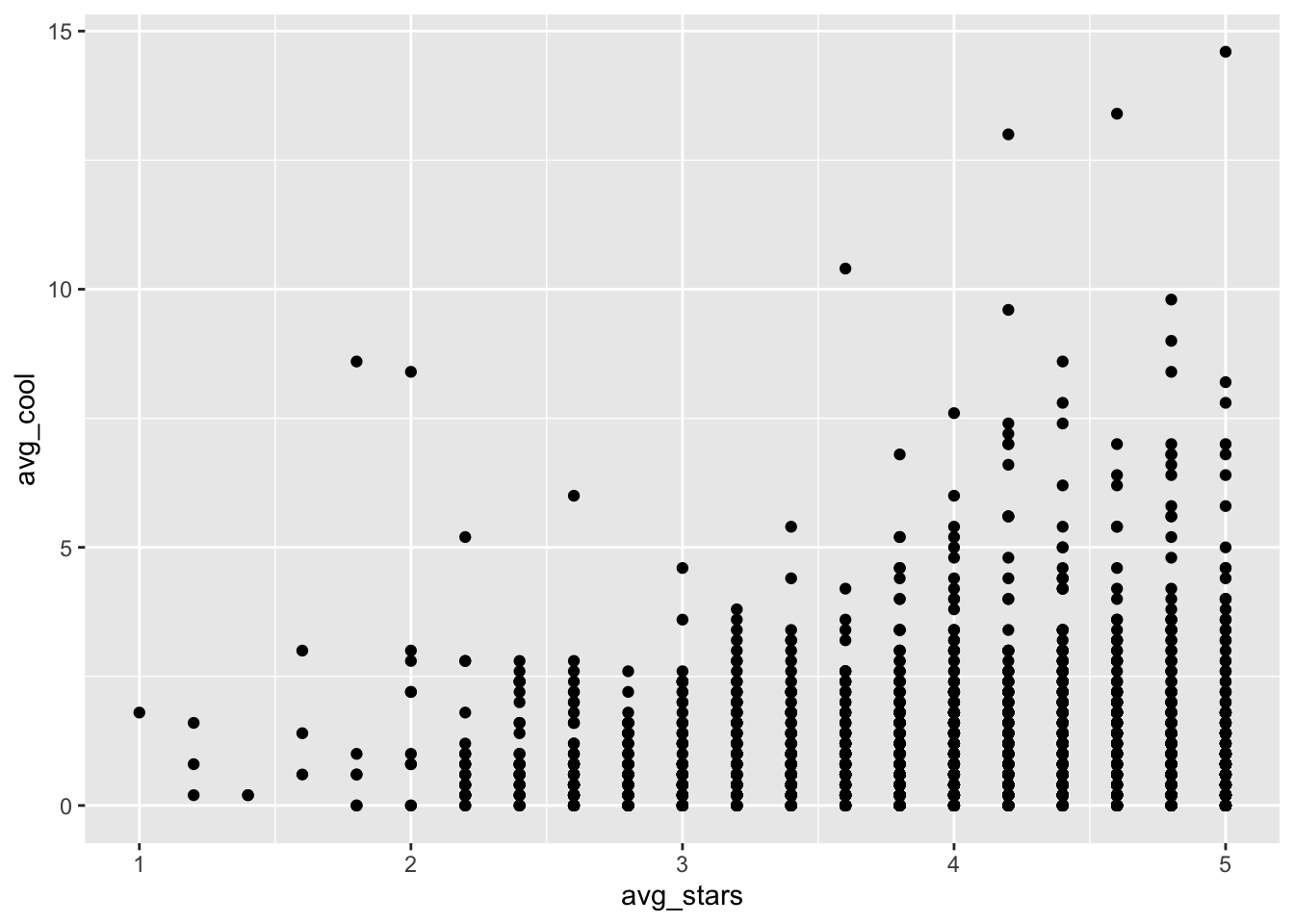
On top of the previous scatterplot, we can add a smoothed line that better identifies the trend between the two variables. With ggformula, we can do this with the pipe %>% operator (will introduce pipes formally in Section ) and call the function gf_smooth() which will add the smoothed line:
gf_point(avg_cool ~ avg_stars, data= t_np) %>% gf_smooth(se=T)## `geom_smooth()` using method = 'gam'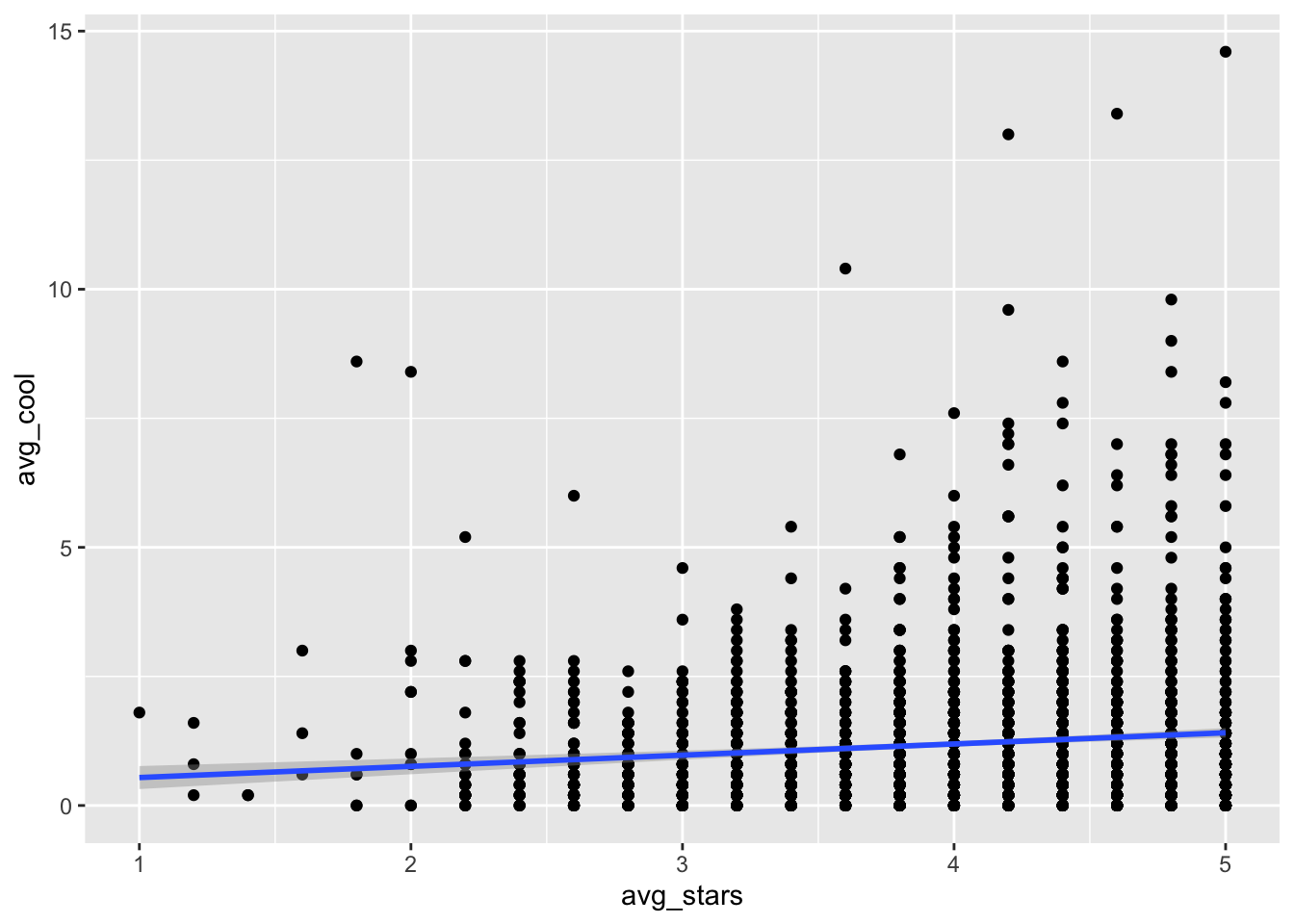
Of course, we can also remove the layer of points, and just focus on the trend line:
gf_smooth(avg_cool ~ avg_stars, data= t_np, se=T) ## `geom_smooth()` using method = 'gam'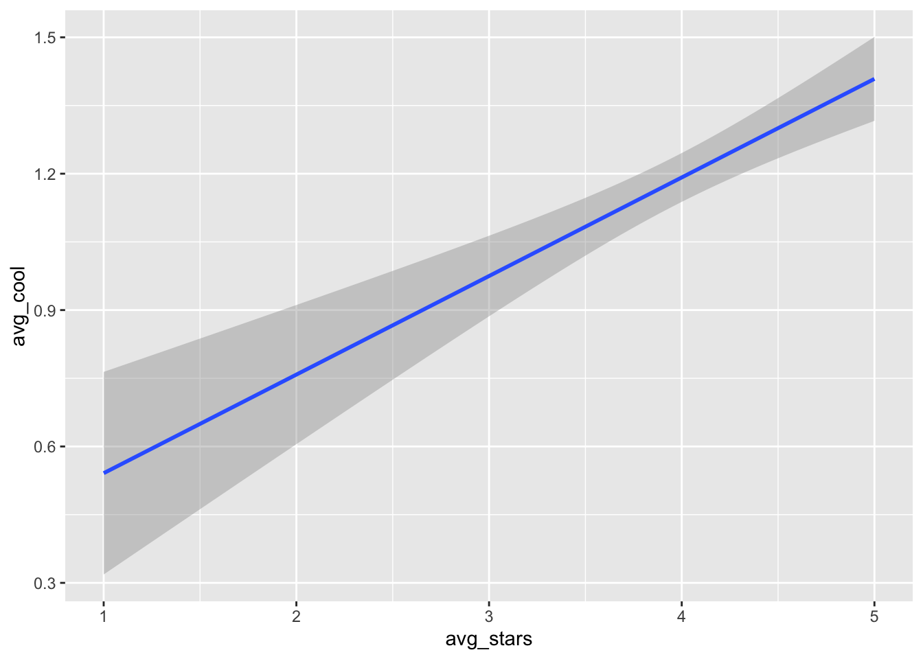
In this last plot, we can see a clear positive relationship between
avg_starsandavg_cool. In the previous figure however, the relationship seemed to be insignificant (i.e., almost zero slope). Just something to think about: different approaches of analysis and visualization can shape different impressions.
Note that inside
gf_smooththere is an argumentse=T. This argument sets the internal variableseof functiongf_smoothto True, so that it can print the error bars arround the smoothed line (the shaded area around the line). Revisit Section 1.6 for more details.
2.3.5 Step 5: Manipulate and enrich the dataset
Finally, we can choose to focus on specific columns of the data, or create new ones.
The functions select() and mutate() from the package dplyr can facilitate these actions.
2.3.5.1 select()
- Are there any variables that we do not want to use?
Often, it might happen that we have to analyze a dataset with thousands of columns. Hence, it might be useful to just isolate the columns that we will most likely need.
To do so, you can use the function select():
st = select(t_np,avg_stars,avg_cool)
st
## # A tibble: 2,324 × 2
## avg_stars avg_cool
## <dbl> <dbl>
## 1 5 7
## 2 4.2 0.8
## 3 4.6 3.6
## 4 4 0.2
## 5 4 0.6
## 6 3.2 0.8
## 7 3.2 0.6
## 8 3 0.4
## 9 4.8 0.4
## 10 4.4 0.4
## # … with 2,314 more rowsIn cases where multiple focal columns start with some identifier, we can use the function starts_with() in combination with the function select().
For instance, to select all columns that start with the letters ‘avg’ we can type:
st = select(t_np,starts_with("avg"))
st
## # A tibble: 2,324 × 4
## avg_stars avg_cool avg_useful avg_funny
## <dbl> <dbl> <dbl> <dbl>
## 1 5 7 8.4 4.4
## 2 4.2 0.8 0.8 0.6
## 3 4.6 3.6 6.2 2
## 4 4 0.2 1.2 1
## 5 4 0.6 1.2 1.4
## 6 3.2 0.8 2.8 0.6
## 7 3.2 0.6 0.6 0.2
## 8 3 0.4 0.4 0
## 9 4.8 0.4 1 0.6
## 10 4.4 0.4 0.4 0.2
## # … with 2,314 more rowsOr, to select columns that ends_with() ‘rs’:
st = select(t_np,ends_with("rs"))
st
## # A tibble: 2,324 × 4
## avg_stars median_stars std_stars Caters
## <dbl> <dbl> <dbl> <lgl>
## 1 5 5 0 NA
## 2 4.2 4 0.837 NA
## 3 4.6 5 0.548 NA
## 4 4 4 1.22 FALSE
## 5 4 4 0.707 TRUE
## 6 3.2 3 0.837 TRUE
## 7 3.2 3 0.837 FALSE
## 8 3 3 1 TRUE
## 9 4.8 5 0.447 NA
## 10 4.4 5 0.894 TRUE
## # … with 2,314 more rows2.3.5.2 mutate()
- Are there new columns (AKA attributes or variables) that we would like to create?
To create a new column we can use the function mutate() of package dplyr.
mutate()adds the new columns at the end of the tibble. For instance:
mt = mutate(t_np,log_avg = log(avg_stars), diff_stars_cool = avg_stars - avg_cool)
select(mt, ends_with("cool"))
## # A tibble: 2,324 × 4
## avg_cool median_cool std_cool diff_stars_cool
## <dbl> <dbl> <dbl> <dbl>
## 1 7 7 4.06 -2
## 2 0.8 1 0.837 3.4
## 3 3.6 3 1.34 1
## 4 0.2 0 0.447 3.8
## 5 0.6 0 0.894 3.4
## 6 0.8 1 0.837 2.4
## 7 0.6 0 0.894 2.6
## 8 0.4 0 0.548 2.6
## 9 0.4 0 0.548 4.4
## 10 0.4 0 0.894 4
## # … with 2,314 more rowsNote that we created a new tibble
mtthat has the new columndiff_stars_cool. Then, by selecting only columns that end withcoolwe were able to clearly see the newly created column at the end.
Finally, we can also get a tibble with only new variables by calling the verb transmute():
mt = transmute(t_np,log_avg = log(avg_stars), diff_stars_cool = avg_stars - avg_cool)
mt
## # A tibble: 2,324 × 2
## log_avg diff_stars_cool
## <dbl> <dbl>
## 1 1.61 -2
## 2 1.44 3.4
## 3 1.53 1
## 4 1.39 3.8
## 5 1.39 3.4
## 6 1.16 2.4
## 7 1.16 2.6
## 8 1.10 2.6
## 9 1.57 4.4
## 10 1.48 4
## # … with 2,314 more rows2.3.6 Summary: How to profile and explore a new dataset
In summary, to profile and explore a new dataset, we can follow these steps:
- Step 1: Understand the columns of the dataset
- Step 2: Identify and handle missing values
- Step 3: Identify patterns in the data
- Step 4: Identify relationships between different columns
- Step 5: Manipulate and enrich the dataset to customize it for your needs
2.4 Pipes: combining multiple operations
Pipes are a powerful tool for clearly expressing a sequence of multiple operations.
For instance, assume that we want to perform the following actions:
- keep only restaurants that have greater than 4
avg stars. - Keep only columns
avg_stars,avg_cool,Price.Range, andAlcohol. - Group by column
Alcohol. - Summarize
avg_stars,avg_cool,Price.RangeperAlcoholgroup.
Based on what we have learned so far, we need to write the following code:
t1 = filter(t_np, avg_stars > 4)
t1 = select(t1,avg_stars, avg_cool, Price.Range, Alcohol)
g = group_by(t1,Alcohol)
summarize(g, mean_stars = mean(avg_stars), mean_cool = mean(avg_cool), mean_price = mean(Price.Range))
## # A tibble: 4 × 4
## Alcohol mean_stars mean_cool mean_price
## <chr> <dbl> <dbl> <dbl>
## 1 beer_and_wine 4.56 1.61 1.73
## 2 full_bar 4.51 1.31 2.18
## 3 none 4.61 1.35 1.31
## 4 <NA> 4.68 1.27 1.79Alternatively, we can use pipes %>%. With pipes, we can perform the same functions in a much simpler, more intuitive way:
t_np %>% filter(avg_stars > 4) %>%
  select(avg_stars, avg_cool, Price.Range, Alcohol) %>%
  group_by(Alcohol) %>%
  summarize(mean_stars = mean(avg_stars), mean_cool = mean(avg_cool), mean_price = mean(Price.Range))
## # A tibble: 4 × 4
## Alcohol mean_stars mean_cool mean_price
## <chr> <dbl> <dbl> <dbl>
## 1 beer_and_wine 4.56 1.61 1.73
## 2 full_bar 4.51 1.31 2.18
## 3 none 4.61 1.35 1.31
## 4 <NA> 4.68 1.27 1.79t_np datarame, and then filter it by keeping only rows with avg_stars > 4, and then select only columns avg_stars, avg_cool, Price.Range, Alcohol, and then group by column Alcohol, and then summarize avg_stars, avg_cool, Price.Range per Alcohol group.
Cmd + Shift + M (Mac) or Ctrl + Shift + M (Windows) inside an R chunk.
For comments, suggestions, errors, and typos, please email me at: kokkodis@bc.edu