6 Case study: A database for NBA games

In this chapter we will design a database for NBA games and we will load it with data basketball-reference.com. We will go over the majority of R functions that we have learned so far, and we will introduce a few new ones that can be particularly useful. Before running the code, check out the focal webpage: https://www.basketball-reference.com/

If you haven’t already, install the package ggthemes:

install.packages('ggthemes')

To start, load the following packages:

library(rvest)
library(tidyverse)
library(ggformula)
library(ggthemes)
library(lubridate)
library(DBI)
library(odbc)
library(RODBC)
pluck = purrr::pluck

The code pluck = purrr::pluck is optional; it allows you to call the function pluck without the purrr:: in front of it.

6.1 Scrape basketball-reference.com

To start, we need to scrape the data. By exploring the website, we can identify that the following URLs store information about the NBA games of a given team:

https://www.basketball-reference.com/teams/[TEAM]/2021_games.html

Let’s explore how we can parse this type of HTML page by focusing on Los Angeles Lakers (LAL):

r = read_html("https://www.basketball-reference.com/teams/LAL/2021_games.html")
r

## {html_document}
## <html data-version="klecko-" data-root="/home/bbr/build" itemscope="" itemtype="https://schema.org/WebSite" lang="en" class="no-js">
## [1] <head>\n<meta http-equiv="Content-Type" content="text/html; charset=UTF-8 ...
## [2] <body class="bbr">\n<div id="wrap">\n  \n  <div id="header" role="banner" ...

6.1.1 `rvest::html_table()`

The structure of the webpage includes multiple tables. Indeed, in this example, we are interested in the available game statistics, which are stored in these tables. Hence, instead of using the SelectorGadget extension, the rvest package has the function html_table that along with HTML tag table allows us to extract all the tables from a webpage:

r1 = r %>% html_nodes("table") %>% html_table()

6.1.2 `purrr::pluck`

This is great, but html_table returns all the available tables within an html web page. What if we wanted a specific table? Luckily, the package purrr that is included in tidyverse has a function called pluck that allows us to access elements from an R object through their index. For instance:

c(1,4,9) %>% purrr::pluck(3)

## [1] 9

In the previous call of pluck I used the name of the package before the function, separated by two consecutive colons, to make sure that I am calling the pluck function from the purrr package. This is important to do because the rvest package has its own pluck function that works a bit differently and it might generate errors in our examples. So because both pluck functions are available in my environment, I need to specify which one of the two I want to use.

(In fact, in my case, because I have used pluck=purrr::pluck in the very begining, I do not really have to use purrr:: front of pluck. I am only using it in case you copy-paste this code.)

Back to our example, let’s assume that I just want to get the first table, I will use the pluck function to do so:

r %>% html_nodes("table") %>% html_table()  %>% purrr::pluck(1)

## # A tibble: 76 × 15
##    G     Date   `Start (ET)` ``    ``     ``    Opponent ``    ``    Tm    Opp  
##    <chr> <chr>  <chr>        <lgl> <chr>  <chr> <chr>    <chr> <chr> <chr> <chr>
##  1 1     Tue, … 10:00p       NA    Box S… ""    Los Ang… L     ""    109   116  
##  2 2     Fri, … 8:00p        NA    Box S… ""    Dallas … W     ""    138   115  
##  3 3     Sun, … 10:00p       NA    Box S… ""    Minneso… W     ""    127   91   
##  4 4     Mon, … 10:00p       NA    Box S… ""    Portlan… L     ""    107   115  
##  5 5     Wed, … 8:30p        NA    Box S… "@"   San Ant… W     ""    121   107  
##  6 6     Fri, … 8:00p        NA    Box S… "@"   San Ant… W     ""    109   103  
##  7 7     Sun, … 6:00p        NA    Box S… "@"   Memphis… W     ""    108   94   
##  8 8     Tue, … 8:00p        NA    Box S… "@"   Memphis… W     ""    94    92   
##  9 9     Thu, … 10:00p       NA    Box S… ""    San Ant… L     ""    109   118  
## 10 10    Fri, … 10:00p       NA    Box S… ""    Chicago… W     ""    117   115  
## # … with 66 more rows, and 4 more variables: W <chr>, L <chr>, Streak <chr>,
## #   Notes <chr>

6.1.3 Repair column names

What columns should we keep from this table? And how can we keep columns that don’t have names? The option .name_repair=c("unique") inside as_tibble can help with rename columns with empty names:

r %>% html_nodes("table") %>% html_table() %>% pluck(1) %>% 
  as_tibble(.name_repair=c("unique")) %>% head

## # A tibble: 6 × 15
##   G     Date    `Start (ET)` ...4  ...5  ...6  Opponent  ...8  ...9  Tm    Opp  
##   <chr> <chr>   <chr>        <lgl> <chr> <chr> <chr>     <chr> <chr> <chr> <chr>
## 1 1     Tue, D… 10:00p       NA    Box … ""    Los Ange… L     ""    109   116  
## 2 2     Fri, D… 8:00p        NA    Box … ""    Dallas M… W     ""    138   115  
## 3 3     Sun, D… 10:00p       NA    Box … ""    Minnesot… W     ""    127   91   
## 4 4     Mon, D… 10:00p       NA    Box … ""    Portland… L     ""    107   115  
## 5 5     Wed, D… 8:30p        NA    Box … "@"   San Anto… W     ""    121   107  
## 6 6     Fri, J… 8:00p        NA    Box … "@"   San Anto… W     ""    109   103  
## # … with 4 more variables: W <chr>, L <chr>, Streak <chr>, Notes <chr>

6.2 Transforming and creating new columns

From the available columns, there are many that store non-relevant information. For instance, ...5, ...5, ...8, etc. Column ...6 stores whether or not a team is visiting or playing at home. This is useful information, so I will rename it to is_away and then drop all the columns that I don’t need:

r %>% html_nodes("table") %>% html_table() %>% pluck(1) %>% 
  as_tibble(.name_repair=c("unique")) %>% 
  rename(is_away=...6) %>% 
    select(-starts_with("..."),-Notes, -G) %>%  head

## # A tibble: 6 × 9
##   Date              `Start (ET)` is_away Opponent Tm    Opp   W     L     Streak
##   <chr>             <chr>        <chr>   <chr>    <chr> <chr> <chr> <chr> <chr> 
## 1 Tue, Dec 22, 2020 10:00p       ""      Los Ang… 109   116   0     1     L 1   
## 2 Fri, Dec 25, 2020 8:00p        ""      Dallas … 138   115   1     1     W 1   
## 3 Sun, Dec 27, 2020 10:00p       ""      Minneso… 127   91    2     1     W 2   
## 4 Mon, Dec 28, 2020 10:00p       ""      Portlan… 107   115   2     2     L 1   
## 5 Wed, Dec 30, 2020 8:30p        "@"     San Ant… 121   107   3     2     W 1   
## 6 Fri, Jan 1, 2021  8:00p        "@"     San Ant… 109   103   4     2     W 2

6.2.1 `dplyr::across`

Many of the columns of our final tibble d are of type character, while they actually need to be numerical. One way to transform these variables to numeric is to use the as.numeric function for each single one of them. However, we can also use the function across inside the mutate function which allows us to apply a third function on multiple columns:

r %>% html_nodes("table") %>% html_table() %>% pluck(1) %>% 
  as_tibble(.name_repair=c("unique")) %>% 
  rename(is_away=...6) %>% 
    select(-starts_with("..."),-Notes, -G) %>% 
  mutate(across(c(Tm,Opp,W,L),as.numeric)) %>% head

## # A tibble: 6 × 9
##   Date              `Start (ET)` is_away Opponent    Tm   Opp     W     L Streak
##   <chr>             <chr>        <chr>   <chr>    <dbl> <dbl> <dbl> <dbl> <chr> 
## 1 Tue, Dec 22, 2020 10:00p       ""      Los Ang…   109   116     0     1 L 1   
## 2 Fri, Dec 25, 2020 8:00p        ""      Dallas …   138   115     1     1 W 1   
## 3 Sun, Dec 27, 2020 10:00p       ""      Minneso…   127    91     2     1 W 2   
## 4 Mon, Dec 28, 2020 10:00p       ""      Portlan…   107   115     2     2 L 1   
## 5 Wed, Dec 30, 2020 8:30p        "@"     San Ant…   121   107     3     2 W 1   
## 6 Fri, Jan 1, 2021  8:00p        "@"     San Ant…   109   103     4     2 W 2

6.2.2 Creating new columns, renaming old ones

On top of the information stored in the data, we want to know which team is visiting and which one is at home. This can be identified implicitly from the is_away column in combination the column Opponent and the fact that we are scraping the Los Angeles Lakers webpage. However, it would be more useful if we could just have a column named home_team and a column named visiting_team:

r %>% html_nodes("table") %>% html_table() %>% pluck(1) %>% 
  as_tibble(.name_repair=c("unique")) %>% 
  rename(is_away=...6) %>% 
    select(-starts_with("..."),-Notes, -G) %>% 
  mutate(across(c(Tm,Opp,W,L),as.numeric)) %>% 
  mutate(home_team = ifelse(is_away=='@',Opponent,'Los Angeles Lakers'), 
         visiting_team = ifelse(is_away!='@',Opponent,'Los Angeles Lakers')) %>% head()

## # A tibble: 6 × 11
##   Date   `Start (ET)` is_away Opponent     Tm   Opp     W     L Streak home_team
##   <chr>  <chr>        <chr>   <chr>     <dbl> <dbl> <dbl> <dbl> <chr>  <chr>    
## 1 Tue, … 10:00p       ""      Los Ange…   109   116     0     1 L 1    Los Ange…
## 2 Fri, … 8:00p        ""      Dallas M…   138   115     1     1 W 1    Los Ange…
## 3 Sun, … 10:00p       ""      Minnesot…   127    91     2     1 W 2    Los Ange…
## 4 Mon, … 10:00p       ""      Portland…   107   115     2     2 L 1    Los Ange…
## 5 Wed, … 8:30p        "@"     San Anto…   121   107     3     2 W 1    San Anto…
## 6 Fri, … 8:00p        "@"     San Anto…   109   103     4     2 W 2    San Anto…
## # … with 1 more variable: visiting_team <chr>

Since I have visiting and home teams, it would be helpful to know the points scored of each one of these. To do so, I can create two new columns: home_team_points, and visiting_team_points:

r %>% html_nodes("table") %>% html_table() %>% pluck(1) %>% 
  as_tibble(.name_repair=c("unique")) %>% 
  rename(is_away=...6) %>% 
    select(-starts_with("..."),-Notes, -G) %>% 
  mutate(across(c(Tm,Opp,W,L),as.numeric)) %>% 
  mutate(home_team = ifelse(is_away=='@',Opponent,'Los Angeles Lakers'), 
         visiting_team = ifelse(is_away!='@',Opponent,'Los Angeles Lakers')) %>%
     mutate(home_team_points = ifelse(Opponent==home_team,Opp,Tm),
        visiting_team_points = ifelse(Opponent!=home_team,Opp,Tm) ) %>% head()

## # A tibble: 6 × 13
##   Date   `Start (ET)` is_away Opponent     Tm   Opp     W     L Streak home_team
##   <chr>  <chr>        <chr>   <chr>     <dbl> <dbl> <dbl> <dbl> <chr>  <chr>    
## 1 Tue, … 10:00p       ""      Los Ange…   109   116     0     1 L 1    Los Ange…
## 2 Fri, … 8:00p        ""      Dallas M…   138   115     1     1 W 1    Los Ange…
## 3 Sun, … 10:00p       ""      Minnesot…   127    91     2     1 W 2    Los Ange…
## 4 Mon, … 10:00p       ""      Portland…   107   115     2     2 L 1    Los Ange…
## 5 Wed, … 8:30p        "@"     San Anto…   121   107     3     2 W 1    San Anto…
## 6 Fri, … 8:00p        "@"     San Anto…   109   103     4     2 W 2    San Anto…
## # … with 3 more variables: visiting_team <chr>, home_team_points <dbl>,
## #   visiting_team_points <dbl>

Some of the columns have names that are not particularly descriptive, so we should rename them appropriately:

– W -> total_wins – L -> total_losses – Streak -> streak – Date -> game_date – Start (ET) -> time

r %>% html_nodes("table") %>% html_table() %>% pluck(1) %>% 
  as_tibble(.name_repair=c("unique")) %>% 
  rename(is_away=...6) %>% 
    select(-starts_with("..."),-Notes, -G) %>% 
  mutate(across(c(Tm,Opp,W,L),as.numeric)) %>% 
  mutate(home_team = ifelse(is_away=='@',Opponent,'Los Angeles Lakers'), 
         visiting_team = ifelse(is_away!='@',Opponent,'Los Angeles Lakers')) %>%
     mutate(home_team_points = ifelse(Opponent==home_team,Opp,Tm),
        visiting_team_points = ifelse(Opponent!=home_team,Opp,Tm) ) %>% 
  rename(total_wins=W,total_losses=L, streak = Streak, game_date = Date, 
         time = `Start (ET)` ) %>% head()

## # A tibble: 6 × 13
##   game_date   time  is_away Opponent     Tm   Opp total_wins total_losses streak
##   <chr>       <chr> <chr>   <chr>     <dbl> <dbl>      <dbl>        <dbl> <chr> 
## 1 Tue, Dec 2… 10:0… ""      Los Ange…   109   116          0            1 L 1   
## 2 Fri, Dec 2… 8:00p ""      Dallas M…   138   115          1            1 W 1   
## 3 Sun, Dec 2… 10:0… ""      Minnesot…   127    91          2            1 W 2   
## 4 Mon, Dec 2… 10:0… ""      Portland…   107   115          2            2 L 1   
## 5 Wed, Dec 3… 8:30p "@"     San Anto…   121   107          3            2 W 1   
## 6 Fri, Jan 1… 8:00p "@"     San Anto…   109   103          4            2 W 2   
## # … with 4 more variables: home_team <chr>, visiting_team <chr>,
## #   home_team_points <dbl>, visiting_team_points <dbl>

6.2.3 A custom function that cleans the tables

The focal HTML page has 2 tables; in addition, I would like to scrape similar webpages for other teams. Since this is a repetetive task, I will need to create a function that takes multiple inputs, including:

the html_file to parse
the table inside the HTML that we are interested in
the team keywords (e.g., LAL)

To do so, I will copy paste the above code and replace any specific information to LAL and table with a relevant parameter:

clear_table = function(html_file, table_position, team){
 html_file %>% html_nodes("table") %>% html_table() %>% pluck(table_position) %>% 
  as_tibble(.name_repair=c("unique")) %>% 
  rename(is_away=...6) %>% 
    select(-starts_with("..."),-Notes, -G) %>% 
  mutate(across(c(Tm,Opp,W,L),as.numeric)) %>% 
  mutate(home_team = ifelse(is_away=='@',Opponent,team), 
         visiting_team = ifelse(is_away!='@',Opponent,team)) %>%
     mutate(home_team_points = ifelse(Opponent==home_team,Opp,Tm),
        visiting_team_points = ifelse(Opponent!=home_team,Opp,Tm) ) %>% 
  rename(total_wins=W,total_losses=L, streak = Streak, game_date = Date, 
         time = `Start (ET)` ) %>% 
     mutate(season=ifelse(table_position==1,'regular','playoffs'))
 
}

Note that even though we did not use the return() function in the previous function, R by default returns the last estimated expression inside the function. So in this case, it will return the desired tibble.

In the previous definition, I also added an extra column named season, which identifies whether the statistics come from the regular season or the playoffs (this is defined by the table position: if the position is 1, then the statistics represent the regular season; otehrwise, they represent the playoffs)

Now we can call the function as follows:

clear_table(r, 2, "Los Angeles Lakers")

## # A tibble: 6 × 14
##   game_date   time   is_away Opponent    Tm   Opp total_wins total_losses streak
##   <chr>       <chr>  <chr>   <chr>    <dbl> <dbl>      <dbl>        <dbl> <chr> 
## 1 Sun, May 2… 3:30p  "@"     Phoenix…    90    99          0            1 L 1   
## 2 Tue, May 2… 10:00p "@"     Phoenix…   109   102          1            1 W 1   
## 3 Thu, May 2… 10:00p ""      Phoenix…   109    95          2            1 W 2   
## 4 Sun, May 3… 3:30p  ""      Phoenix…    92   100          2            2 L 1   
## 5 Tue, Jun 1… 10:00p "@"     Phoenix…    85   115          2            3 L 2   
## 6 Thu, Jun 3… 10:30p ""      Phoenix…   100   113          2            4 L 3   
## # … with 5 more variables: home_team <chr>, visiting_team <chr>,
## #   home_team_points <dbl>, visiting_team_points <dbl>, season <chr>

6.2.4 `dplyr:bind_rows`

We can combine the two with the function bind_rows():

clear_table(r, 1, "Los Angeles Lakers") %>% bind_rows(clear_table(r, 2, "Los Angeles Lakers"))

## # A tibble: 82 × 14
##    game_date  time  is_away Opponent     Tm   Opp total_wins total_losses streak
##    <chr>      <chr> <chr>   <chr>     <dbl> <dbl>      <dbl>        <dbl> <chr> 
##  1 Tue, Dec … 10:0… ""      Los Ange…   109   116          0            1 L 1   
##  2 Fri, Dec … 8:00p ""      Dallas M…   138   115          1            1 W 1   
##  3 Sun, Dec … 10:0… ""      Minnesot…   127    91          2            1 W 2   
##  4 Mon, Dec … 10:0… ""      Portland…   107   115          2            2 L 1   
##  5 Wed, Dec … 8:30p "@"     San Anto…   121   107          3            2 W 1   
##  6 Fri, Jan … 8:00p "@"     San Anto…   109   103          4            2 W 2   
##  7 Sun, Jan … 6:00p "@"     Memphis …   108    94          5            2 W 3   
##  8 Tue, Jan … 8:00p "@"     Memphis …    94    92          6            2 W 4   
##  9 Thu, Jan … 10:0… ""      San Anto…   109   118          6            3 L 1   
## 10 Fri, Jan … 10:0… ""      Chicago …   117   115          7            3 W 1   
## # … with 72 more rows, and 5 more variables: home_team <chr>,
## #   visiting_team <chr>, home_team_points <dbl>, visiting_team_points <dbl>,
## #   season <chr>

6.3 Repetitive scraping

Our goal is not to just analyze the LA Lakers, but instead, to compare the performance of multiple teams. Hence, it would be useful to create a custom function that extracts the above info for any team we care about. Then, we would be able to call that function repeatedly for different teams.

6.3.1 Lists as dictionaries

If you notice, we need the team’s code “LAL” and the team’s full name “Los Angeles Lakers” to scrape and clean the data. To do this for multiple teams, we will need to define a structure that will map each team code to the team’s full name. In programming, such structures are called dictionaries; in R, we will use the name attribute of a list as follows:

team_dict = list(LAL="Los Angeles Lakers", BOS='Boston Celtics', MIA="Miami Heat", DEN = "Denver Nuggets")
names(team_dict)

## [1] "LAL" "BOS" "MIA" "DEN"

Now we can access the full name of a team by providing the team code:

team_dict[['LAL']]

## [1] "Los Angeles Lakers"

Or through the pluck function:

team_dict %>% purrr::pluck(1)

## [1] "Los Angeles Lakers"

The final function will look as follows:

scrape_and_clean_team = function(team_code){
  r = read_html(paste("https://www.basketball-reference.com/teams/",team_code,"/2021_games.html",sep=""))
  cur_team = team_dict[[team_code]]
  clear_table(r, 1,cur_team ) %>% bind_rows(clear_table(r, 2, cur_team)) %>% 
    mutate(query_team=cur_team)
}

In the previous definition, I also added an extra column named query_team, which is useful to identify for which team the columns total_wins, total_losses, and streak refer to.

Now we can call this function for multiple teams with the function map_dfr:

c("MIA", "LAL", "BOS", "DEN") %>% map_dfr(scrape_and_clean_team) -> d
d %>% select(query_team) %>% distinct

## # A tibble: 4 × 1
##   query_team        
##   <chr>             
## 1 Miami Heat        
## 2 Los Angeles Lakers
## 3 Boston Celtics    
## 4 Denver Nuggets

6.3.2 `lubridate::as_date(,format)`

If we look at our final tibble d we will see that the game_date column has a format that is not recognized as a date format by R. It would have been nice to be able to transform this format into an actual date type. Fortunately, we can do this with the function as_date that we have used in the past, along with its parameter format that we can set to match any specific date format:

as_date("Wed, Oct 23, 2021", format="%a, %b %d, %Y")

## [1] "2021-10-23"

An explanation of the format keywords can be found here: https://rdrr.io/r/base/strptime.html

We can apply this format to the column game_date and transform it to date type:

d$game_date = as_date(d$game_date, format="%a, %b %d, %Y")
d %>% select(game_date) %>% head

## # A tibble: 6 × 1
##   game_date 
##   <date>    
## 1 2020-12-23
## 2 2020-12-25
## 3 2020-12-29
## 4 2020-12-30
## 5 2021-01-01
## 6 2021-01-04

6.4 Designing a relevant database

Now we will use the scraped data to design and fill a relevant database.

6.4.1 An ERD

First, we will need to create an ERD. The main questions we will need to answer are the following:

Which are the entities?
What are their primary keys?
What are their relationships?

Some clarifications:

Each team plays multiple games; each game is played between two teams.
Each game has various statistics along with location and time info.
home_team and visiting_team –> represent “teams”

There are three clear conceptual entities:

team
game
team_in_game

Conceptually, the entity team stores information about the each team (each team appear in a single row). The team name (or the team code) can be used as primary keys. The entity game info will store details about the location and date info for each game. Each game should have a unique ID that will serve as primary key. Each row in the game should represent a single game.

Finally, the entity team_in_game will store the performance of each team in a single game. Each row, will represent the statistics of a team in a game. Game ID and team name can serve as a composite primary key (as each team plays each game once).

The team_in_game is a relationship table that connect the entities team and game. Each team can participate in multiple games , hence the relationship between team and team_in_game is one to many. Similarly, each game will appear twice in team_in_game, hence the relationship between game and team_in_game will also be one to many.

The final ERD is as follows:

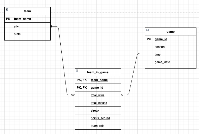
Figure 6.1: An Entity Relationship diagram of the NBA database.

6.4.2 Creating the tables

Based on the above ERD, we will create our tables. First, we will need to connect to the database:

con = DBI::dbConnect(odbc::odbc(), 
                    Driver= "MySQL", 
                    Server='mysql-isys3350.bc.edu', 
                    UID='your_username', 
                    PWD= 'your_password',
                    Port= 3306, 
                    Database = "kokkodis_student_db")

Note the extra parameter Database above is needed in order to use the function dbWriteTable in Section~ 6.5.

CREATE TABLE kokkodis_student_db.team (
    team_name VARCHAR(100),
    city VARCHAR(50),
    state VARCHAR(50),
    PRIMARY KEY (team_name)
);

CREATE TABLE kokkodis_student_db.game (
    game_id VARCHAR(100),
    season VARCHAR(50),
    time VARCHAR(50),
      game_date DATE,
    PRIMARY KEY (game_id)
);

CREATE TABLE kokkodis_student_db.team_in_game (
    game_id VARCHAR(100),
    team_name VARCHAR(100),
    PRIMARY KEY (game_id,team_name),
      total_wins INT,
      total_losses INT,
      streak VARCHAR(10),
      points_scored INT,
      is_team_home VARCHAR(1),
    CONSTRAINT fk_game
    FOREIGN KEY (game_id)
    REFERENCES kokkodis_student_db.game (game_id),
    CONSTRAINT fk_team
    FOREIGN KEY (team_name)
    REFERENCES kokkodis_student_db.team (team_name)
);

Note the definition of the two foreign keys in table kokkodis_student_db.team_in_game.

6.5 Load data from df to db

Next, we will need to create the tables from our main tibble d.

6.5.1 Loading table `team`

We will start with table team, which has three columns: team_name, city, and state. We do not have any information about the city and state of each team, so we will fill these columns with missing values NA.

d %>% select(home_team) %>% distinct %>% mutate(city=NA, state=NA) %>% rename(team_name=home_team)-> team
team %>% head

## # A tibble: 6 × 3
##   team_name          city  state
##   <chr>              <lgl> <lgl>
## 1 Orlando Magic      NA    NA   
## 2 Miami Heat         NA    NA   
## 3 Dallas Mavericks   NA    NA   
## 4 Washington Wizards NA    NA   
## 5 Philadelphia 76ers NA    NA   
## 6 Toronto Raptors    NA    NA

We can now call the function dbWriteTable to load the data to the database table. Function dbWriteTable has the following syntax:

dbWriteTable(connection, database_table_name, tibble_name, append = T)

Hence, in our example:

dbWriteTable(con,"team", team, append = T)

Note that I am using the option append=T. Without it, the dbWriteTable will try to create the table team. Because the table team already exists, it will raise an error.

For the dbWriteTable command to work, you need to make sure that (1) you have chosen a database inside the DBI::dbConnect, and (2) that the column names of your tibble match the column names of your database table.

Let’s verify that we have actually loaded the data:

select * from kokkodis_student_db.team;

Table 6.1: Displaying records 1 - 10
team_name	city	state
Atlanta Hawks	NA	NA
Boston Celtics	NA	NA
Brooklyn Nets	NA	NA
Charlotte Hornets	NA	NA
Chicago Bulls	NA	NA
Cleveland Cavaliers	NA	NA
Dallas Mavericks	NA	NA
Denver Nuggets	NA	NA
Detroit Pistons	NA	NA
Golden State Warriors	NA	NA

6.5.2 Loading table `game`

Similar to before:

d %>%   mutate(game_id = paste(game_date, home_team)) -> d
d %>% 
  select(game_id,time,game_date,season) %>% distinct -> game
game #%>% head

## # A tibble: 306 × 4
##    game_id                       time   game_date  season 
##    <chr>                         <chr>  <date>     <chr>  
##  1 2020-12-23 Orlando Magic      7:00p  2020-12-23 regular
##  2 2020-12-25 Miami Heat         12:00p 2020-12-25 regular
##  3 2020-12-29 Miami Heat         7:30p  2020-12-29 regular
##  4 2020-12-30 Miami Heat         7:30p  2020-12-30 regular
##  5 2021-01-01 Dallas Mavericks   7:00p  2021-01-01 regular
##  6 2021-01-04 Miami Heat         7:30p  2021-01-04 regular
##  7 2021-01-06 Miami Heat         7:30p  2021-01-06 regular
##  8 2021-01-09 Washington Wizards 7:00p  2021-01-09 regular
##  9 2021-01-12 Philadelphia 76ers 7:00p  2021-01-12 regular
## 10 2021-01-14 Philadelphia 76ers 7:00p  2021-01-14 regular
## # … with 296 more rows

Note that we created a new column game_id that combines the game_date with the home_team to generate a unique identifies for each game (since each team plays once at each date).

If we look a little closer into this table, we will find some missing values:

game %>% summary

##    game_id              time             game_date             season         
##  Length:306         Length:306         Min.   :2020-12-22   Length:306        
##  Class :character   Class :character   1st Qu.:2021-02-01   Class :character  
##  Mode  :character   Mode  :character   Median :2021-03-16   Mode  :character  
##                                        Mean   :2021-03-13                     
##                                        3rd Qu.:2021-04-23                     
##                                        Max.   :2021-06-13                     
##                                        NA's   :5

Let’s investigate why:

game %>% filter(is.na(game_date))

## # A tibble: 5 × 4
##   game_id               time       game_date season  
##   <chr>                 <chr>      <date>    <chr>   
## 1 NA Miami Heat         Start (ET) NA        regular 
## 2 NA Los Angeles Lakers Start (ET) NA        regular 
## 3 NA Boston Celtics     Start (ET) NA        regular 
## 4 NA Denver Nuggets     Start (ET) NA        regular 
## 5 NA Denver Nuggets     Start (ET) NA        playoffs

Base on the above, these are filler rows (within the table) that we do not need. Hence, we will drop these rows:

game = game %>% filter(!is.na(game_date))

dbWriteTable(con,"game",game, append=T)

select * from game;

Table 6.2: Displaying records 1 - 10
game_id	season	time	game_date
2020-12-22 Los Angeles Lakers	regular	10:00p	2020-12-22
2020-12-23 Boston Celtics	regular	7:30p	2020-12-23
2020-12-23 Denver Nuggets	regular	9:00p	2020-12-23
2020-12-23 Orlando Magic	regular	7:00p	2020-12-23
2020-12-25 Boston Celtics	regular	5:00p	2020-12-25
2020-12-25 Denver Nuggets	regular	10:30p	2020-12-25
2020-12-25 Los Angeles Lakers	regular	8:00p	2020-12-25
2020-12-25 Miami Heat	regular	12:00p	2020-12-25
2020-12-27 Indiana Pacers	regular	8:00p	2020-12-27
2020-12-27 Los Angeles Lakers	regular	10:00p	2020-12-27

6.5.3 Loading table `team_in_game`

The final table team_in_game is a little bit more complex. The reason is that in our original tibble d, each row includes two teams: the home_team and the visiting_team. However, the team_in_game table decomposes this such as each row includes a single team (either the home team or the visiting team).

The first step we need to do is to transform our tibble such that each row represents one team. The function pivot_longer takes multiple columns and puts their values under two columns, one that identifies the original column name (parameter names_to) and one that identifies the value (parameter values_to):

d %>% pivot_longer(cols = c('home_team','visiting_team'), names_to = "is_team_home", values_to = "team_name") -> dl
dl

## # A tibble: 656 × 16
##    game_date  time   is_away Opponent    Tm   Opp total_wins total_losses streak
##    <date>     <chr>  <chr>   <chr>    <dbl> <dbl>      <dbl>        <dbl> <chr> 
##  1 2020-12-23 7:00p  "@"     Orlando…   107   113          0            1 L 1   
##  2 2020-12-23 7:00p  "@"     Orlando…   107   113          0            1 L 1   
##  3 2020-12-25 12:00p ""      New Orl…   111    98          1            1 W 1   
##  4 2020-12-25 12:00p ""      New Orl…   111    98          1            1 W 1   
##  5 2020-12-29 7:30p  ""      Milwauk…    97   144          1            2 L 1   
##  6 2020-12-29 7:30p  ""      Milwauk…    97   144          1            2 L 1   
##  7 2020-12-30 7:30p  ""      Milwauk…   119   108          2            2 W 1   
##  8 2020-12-30 7:30p  ""      Milwauk…   119   108          2            2 W 1   
##  9 2021-01-01 7:00p  "@"     Dallas …    83    93          2            3 L 1   
## 10 2021-01-01 7:00p  "@"     Dallas …    83    93          2            3 L 1   
## # … with 646 more rows, and 7 more variables: home_team_points <dbl>,
## #   visiting_team_points <dbl>, season <chr>, query_team <chr>, game_id <chr>,
## #   is_team_home <chr>, team_name <chr>

Next, we need to associate columns total_wins, total_losses, and streak with the query_team:

dl %>%  filter(team_name == query_team) %>% select(team_name, game_id, total_wins, total_losses, streak,  home_team_points, is_team_home, visiting_team_points)  -> dl1
dl1 %>% head

## # A tibble: 6 × 8
##   team_name  game_id total_wins total_losses streak home_team_points is_team_home
##   <chr>      <chr>        <dbl>        <dbl> <chr>             <dbl> <chr>       
## 1 Miami Heat 2020-1…          0            1 L 1                 113 visiting_te…
## 2 Miami Heat 2020-1…          1            1 W 1                 111 home_team   
## 3 Miami Heat 2020-1…          1            2 L 1                  97 home_team   
## 4 Miami Heat 2020-1…          2            2 W 1                 119 home_team   
## 5 Miami Heat 2021-0…          2            3 L 1                  93 visiting_te…
## 6 Miami Heat 2021-0…          3            3 W 1                 118 home_team   
## # … with 1 more variable: visiting_team_points <dbl>

For the teams that we did not query, we do not have any info about their total_wins, total_losses, and streak. Hence, for those teams, we will fill those columns with missing values:

dl %>%  filter(team_name != query_team) %>% select(team_name, game_id, total_wins, total_losses, streak,  home_team_points, is_team_home, visiting_team_points) %>% 
  mutate(total_losses=NA,total_wins=NA,streak=NA)->dl2
dl2 %>% head

## # A tibble: 6 × 8
##   team_name game_id total_wins total_losses streak home_team_points is_team_home
##   <chr>     <chr>   <lgl>      <lgl>        <lgl>             <dbl> <chr>       
## 1 Orlando … 2020-1… NA         NA           NA                  113 home_team   
## 2 New Orle… 2020-1… NA         NA           NA                  111 visiting_te…
## 3 Milwauke… 2020-1… NA         NA           NA                   97 visiting_te…
## 4 Milwauke… 2020-1… NA         NA           NA                  119 visiting_te…
## 5 Dallas M… 2021-0… NA         NA           NA                   93 home_team   
## 6 Oklahoma… 2021-0… NA         NA           NA                  118 visiting_te…
## # … with 1 more variable: visiting_team_points <dbl>

Now we can combine the two with bind_rows, and update the column names to much those in the table:

dl1 %>%   bind_rows(dl2) %>%
  mutate(points_scored = ifelse(is_team_home=='visiting_team', visiting_team_points, home_team_points)) %>% 
  select(-c(visiting_team_points,home_team_points)) %>% 
  mutate(is_team_home =  ifelse(is_team_home=='visiting_team','N', 'Y')) %>% 
  distinct -> team_in_game
team_in_game

## # A tibble: 638 × 7
##    team_name  game_id  total_wins total_losses streak is_team_home points_scored
##    <chr>      <chr>         <dbl>        <dbl> <chr>  <chr>                <dbl>
##  1 Miami Heat 2020-12…          0            1 L 1    N                      107
##  2 Miami Heat 2020-12…          1            1 W 1    Y                      111
##  3 Miami Heat 2020-12…          1            2 L 1    Y                       97
##  4 Miami Heat 2020-12…          2            2 W 1    Y                      119
##  5 Miami Heat 2021-01…          2            3 L 1    N                       83
##  6 Miami Heat 2021-01…          3            3 W 1    Y                      118
##  7 Miami Heat 2021-01…          3            4 L 1    Y                      105
##  8 Miami Heat 2021-01…          4            4 W 1    N                      128
##  9 Miami Heat 2021-01…          4            5 L 1    N                      134
## 10 Miami Heat 2021-01…          4            6 L 2    N                      108
## # … with 628 more rows

Let’s check this tibble:

team_in_game %>% summary

##   team_name           game_id            total_wins     total_losses  
##  Length:638         Length:638         Min.   : 0.00   Min.   : 0.00  
##  Class :character   Class :character   1st Qu.: 7.00   1st Qu.: 6.00  
##  Mode  :character   Mode  :character   Median :19.00   Median :15.00  
##                                        Mean   :19.28   Mean   :14.88  
##                                        3rd Qu.:31.00   3rd Qu.:23.00  
##                                        Max.   :47.00   Max.   :36.00  
##                                        NA's   :323     NA's   :323    
##     streak          is_team_home       points_scored  
##  Length:638         Length:638         Min.   : 75.0  
##  Class :character   Class :character   1st Qu.:102.0  
##  Mode  :character   Mode  :character   Median :110.0  
##                                        Mean   :110.3  
##                                        3rd Qu.:119.0  
##                                        Max.   :147.0  
##                                        NA's   :8

Column points_scored should not have missing values, so we will remove those:

team_in_game= team_in_game %>% filter(!is.na(points_scored))
team_in_game

## # A tibble: 630 × 7
##    team_name  game_id  total_wins total_losses streak is_team_home points_scored
##    <chr>      <chr>         <dbl>        <dbl> <chr>  <chr>                <dbl>
##  1 Miami Heat 2020-12…          0            1 L 1    N                      107
##  2 Miami Heat 2020-12…          1            1 W 1    Y                      111
##  3 Miami Heat 2020-12…          1            2 L 1    Y                       97
##  4 Miami Heat 2020-12…          2            2 W 1    Y                      119
##  5 Miami Heat 2021-01…          2            3 L 1    N                       83
##  6 Miami Heat 2021-01…          3            3 W 1    Y                      118
##  7 Miami Heat 2021-01…          3            4 L 1    Y                      105
##  8 Miami Heat 2021-01…          4            4 W 1    N                      128
##  9 Miami Heat 2021-01…          4            5 L 1    N                      134
## 10 Miami Heat 2021-01…          4            6 L 2    N                      108
## # … with 620 more rows

6.5.4 Removing duplicates with the `group_by` trick

Let’s check if there are any duplicate keys:

team_in_game %>% count(game_id, team_name) %>% filter(n > 1)

## # A tibble: 28 × 3
##    game_id                       team_name              n
##    <chr>                         <chr>              <int>
##  1 2021-01-06 Miami Heat         Boston Celtics         2
##  2 2021-01-06 Miami Heat         Miami Heat             2
##  3 2021-01-27 Miami Heat         Denver Nuggets         2
##  4 2021-01-27 Miami Heat         Miami Heat             2
##  5 2021-01-30 Boston Celtics     Boston Celtics         2
##  6 2021-01-30 Boston Celtics     Los Angeles Lakers     2
##  7 2021-02-04 Los Angeles Lakers Denver Nuggets         2
##  8 2021-02-04 Los Angeles Lakers Los Angeles Lakers     2
##  9 2021-02-14 Denver Nuggets     Denver Nuggets         2
## 10 2021-02-14 Denver Nuggets     Los Angeles Lakers     2
## # … with 18 more rows

Let’s try to understand why:

team_in_game %>% filter(game_id=='2021-01-06 Miami Heat' & team_name =='Boston Celtics')

## # A tibble: 2 × 7
##   team_name      game_id total_wins total_losses streak is_team_home points_scored
##   <chr>          <chr>        <dbl>        <dbl> <chr>  <chr>                <dbl>
## 1 Boston Celtics 2021-0…          6            3 W 3    N                      107
## 2 Boston Celtics 2021-0…         NA           NA <NA>   N                      107

In cases like these, we want to keep the first row, which includes more info about the Boston Celtics (i.e., the row that originated from scraping the BOS web page). A nice trick to do this is to use group_by:

team_in_game %>% group_by(game_id, team_name, points_scored, is_team_home) %>%
  summarize(
    n = n(),
    total_wins =
      ifelse(n == 1, NA, max(total_wins, na.rm = T)),
    total_losses =
      ifelse(n == 1, NA, max(total_losses, na.rm = T)),
    streak = ifelse(n == 1, NA, max(streak, na.rm = T))
  ) %>%
  ungroup %>% distinct -> team_in_game
team_in_game

## # A tibble: 602 × 8
##    game_id   team_name  points_scored is_team_home     n total_wins total_losses
##    <chr>     <chr>              <dbl> <chr>        <int>      <dbl>        <dbl>
##  1 2020-12-… Los Angel…           116 N                1         NA           NA
##  2 2020-12-… Los Angel…           109 Y                1         NA           NA
##  3 2020-12-… Boston Ce…           122 Y                1         NA           NA
##  4 2020-12-… Milwaukee…           121 N                1         NA           NA
##  5 2020-12-… Denver Nu…           122 Y                1         NA           NA
##  6 2020-12-… Sacrament…           124 N                1         NA           NA
##  7 2020-12-… Miami Heat           107 N                1         NA           NA
##  8 2020-12-… Orlando M…           113 Y                1         NA           NA
##  9 2020-12-… Boston Ce…            95 Y                1         NA           NA
## 10 2020-12-… Brooklyn …           123 N                1         NA           NA
## # … with 592 more rows, and 1 more variable: streak <chr>

Explore what happens if I do not include the ifelse checks in the previous piece of code. In general, try to understand how this code works.

Finally, we are ready to load the team_in_game tibble into the team_in_game table in our database:

dbWriteTable(con,"team_in_game", team_in_game %>% select(-n), append = T)

select * from kokkodis_student_db.team_in_game;

Table 6.3: Displaying records 1 - 10
game_id	team_name	total_wins	total_losses	streak	points_scored	is_team_home
2020-12-22 Los Angeles Lakers	Los Angeles Clippers	NA	NA	NA	116	N
2020-12-22 Los Angeles Lakers	Los Angeles Lakers	NA	NA	NA	109	Y
2020-12-23 Boston Celtics	Boston Celtics	NA	NA	NA	122	Y
2020-12-23 Boston Celtics	Milwaukee Bucks	NA	NA	NA	121	N
2020-12-23 Denver Nuggets	Denver Nuggets	NA	NA	NA	122	Y
2020-12-23 Denver Nuggets	Sacramento Kings	NA	NA	NA	124	N
2020-12-23 Orlando Magic	Miami Heat	NA	NA	NA	107	N
2020-12-23 Orlando Magic	Orlando Magic	NA	NA	NA	113	Y
2020-12-25 Boston Celtics	Boston Celtics	NA	NA	NA	95	Y
2020-12-25 Boston Celtics	Brooklyn Nets	NA	NA	NA	123	N

6.6 Queries and plots

Let’s draw the distributions of points for Boston Celtics and Miami Heat:

query = 'SELECT points_scored, team_name FROM kokkodis_student_db.team_in_game WHERE team_name in ("Miami Heat", "Boston Celtics");'
t = dbGetQuery(con,query) %>% as_tibble
t

## # A tibble: 154 × 2
##    points_scored team_name     
##            <int> <chr>         
##  1           122 Boston Celtics
##  2           107 Miami Heat    
##  3            95 Boston Celtics
##  4           111 Miami Heat    
##  5           107 Boston Celtics
##  6           116 Boston Celtics
##  7            97 Miami Heat    
##  8           126 Boston Celtics
##  9           119 Miami Heat    
## 10            83 Miami Heat    
## # … with 144 more rows

Package ggthemes allows us to plot our graphs within different themes. For instance, we can use the economist theme:

t %>% gf_density(~points_scored, fill=~team_name) +
  theme_economist()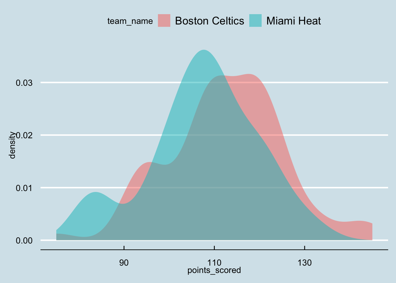

If you start typing theme_ the autocomplete will show you all the available themes from the package ggthemes.

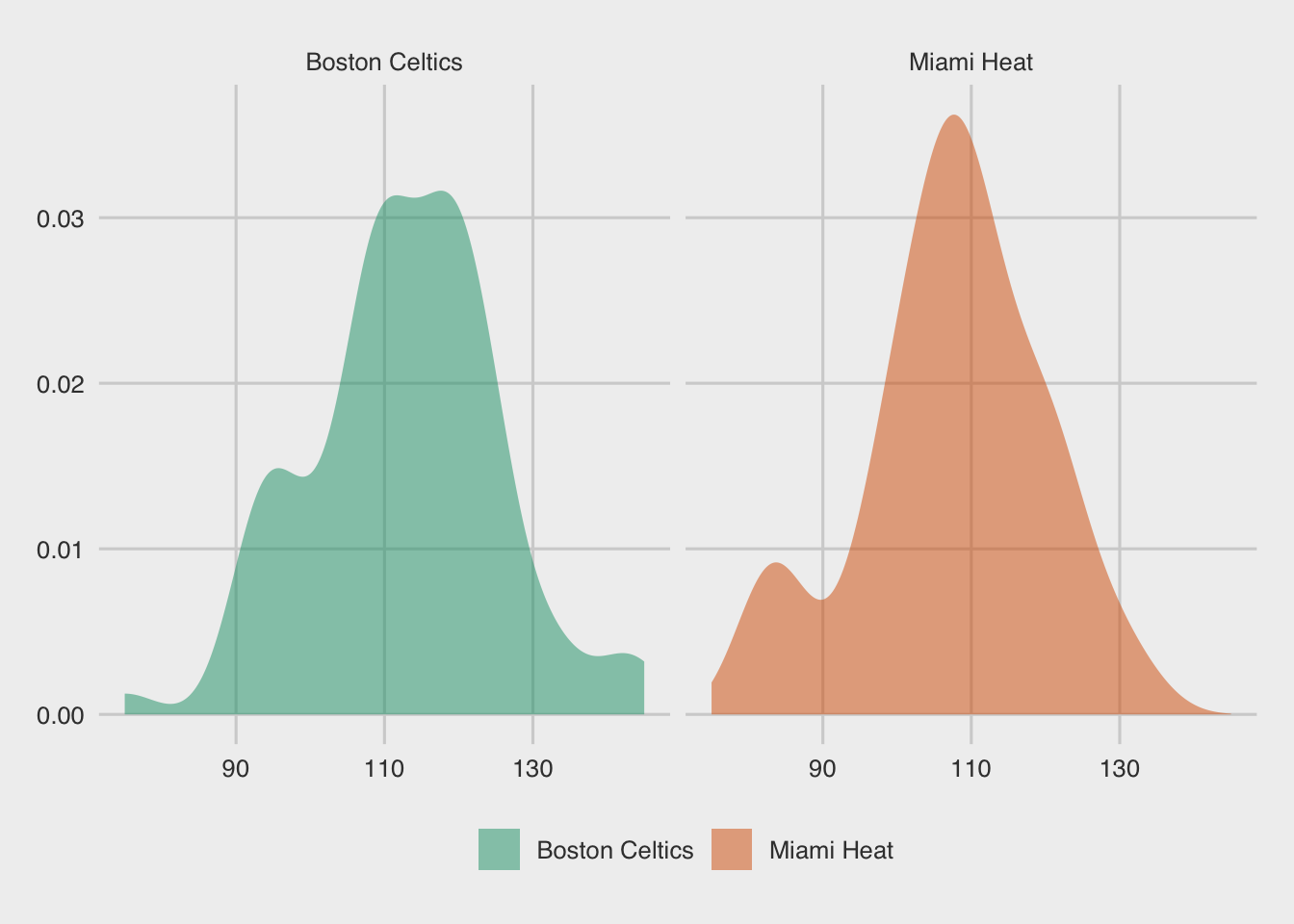
6.6.1 `facet_wrap`

Now let’s plot the distributions of the margin of victory for the four teams. The function facet_wrap allows us to visualize the distribution of each team in a separate plot next to each other. The functions scale_fill_brewer allows us to use predetermined color palettes. You can find these palettes here: https://rdrr.io/cran/RColorBrewer/man/ColorBrewer.html

t %>% gf_density(~points_scored, fill=~team_name) +
   theme_fivethirtyeight()+facet_wrap(~team_name, ncol = 2) +
  scale_fill_brewer(palette = "Dark2") + theme(legend.title = element_blank())

6 Case study: A database for NBA games

6.1 Scrape basketball-reference.com

6.1.1 rvest::html_table()

6.1.2 purrr::pluck