11 Basic text analytics
In this chapter we will go over some basic text analytics approaches, including regular expressions, bag of words, and sentiment analysis. We will present how to handle text primarily in R but also with some advanced SQL functions.
11.1 Regular expressions
Regular expressions allow us to match and extract useful patterns from unstructured text.
The regular expression functions that we will use come from the package stringr, which is included in tidyverse:
library(tidyverse)
library(DBI)
library(odbc)
library(RODBC)
11.1.1 Atoms
An atom specifies what text is to be matched and where it is to be found. There are four types of atoms:
- a single character
- a dot
- a class
- an anchor
To match patterns, we will use the function str_detect.
11.1.1.1 A single character
The following tests whether the single characters “L” and “S” are found in “HELLO”:
str_detect("HELLO","L")## [1] TRUEstr_detect("HELLO","S")## [1] FALSE11.1.1.2 The dot
The dot matches any single character:
str_detect("HELLO",".")## [1] TRUEstr_detect("HELLO","H.")## [1] TRUEstr_detect("HELLO","h.")## [1] FALSEstr_detect("HELLO",".L.O")## [1] TRUE11.1.1.3 Class
A class matching returns TRUE if any of the single characters inside the class is found in the examined string.
We define a class by using brackets. For instance, [ABL] matches A, B, or L:
str_detect("HELLO","[ABL]")## [1] TRUEstr_detect("HELLO A or HELLO B","[AB]")## [1] TRUERanges are popular class atoms:
str_detect("HELLO A or HELLO B","[0-9]")## [1] FALSEstr_detect("HELLO A HELLO B","[a-z]")## [1] FALSEstr_detect("HELLO A HELLO B","[a-zA-Z]")## [1] TRUEstr_detect("HELLO A HELLO B.",".")## [1] TRUE11.1.1.4 Anchor
An anchor atom specifies the position in the string where a match must occurs. A caret (^) identifies the beginning of the line, while a dollar sign ($) the end of a line.
str_detect("HELLO A HELLO B.","^H")## [1] TRUEstr_detect("HELLO A HELLO B.","^H$")## [1] FALSEstr_detect("HELLO A HELLO B.",".$")## [1] TRUEstr_detect("HELLO A or HELLO B","[^0-9]")## [1] TRUE
Note that a caret within a bracket represents a logical NOT. Hence,
[^0-9]meansNOT a digit.
11.1.2 Operators
Operators in regular expressions combine atoms. An operator can be:
- a sequence of atoms
- alternation of atoms
- repetition of atoms
- grouping of atoms.
11.1.2.1 Sequence
A sequence of atoms:
str_detect("HELLO A HELLO B.","HELLO")## [1] TRUEstr_detect("HELLO A HELLO B.","[A-Z][A-Z]")## [1] TRUEstr_detect("HELLO A 6 4 HELLO B.","[0-9][0-9]")## [1] FALSE11.1.2.2 Alternation
Alternation is similar to logical OR:
str_detect("HELLO A HELLO B.","HELLO|A")## [1] TRUEstr_detect("HELLO A HELLO B.","[A-Z]|[0-9]")## [1] TRUEstr_detect("HELLO A8 HELLO B.","[A-Za-z][0-9]|[0-9]")## [1] TRUE11.1.2.3 Repitition
The repetition operator is represented by curly brackets. For instance {m,n} matches the atoms or expressions that appear before the brackets from m to n times:
str_detect("HELLO A HELLO B.","L{3,4}")## [1] FALSEstr_detect("",".*")## [1] TRUEstr_detect("HELLO A","H+")## [1] TRUEstr_detect("HELLO A","K?")## [1] TRUEstr_detect("HELLO A","L?")## [1] TRUE11.1.2.4 Grouping
Grouping is represented by parentheses and identifies the expression that a subsequent operator will be applied to:
str_detect("HELLO A","(LO)?")## [1] TRUEstr_detect("HELLO A","(LOL)+")## [1] FALSEstr_detect("HELLO A","(LOL)+|(LO)*")## [1] TRUEstr_detect("HELLO A","(LOL)+|([0-9]|A){2,5}")## [1] FALSE11.1.3 An example that extracts information from news titles
Load the dataset newsTitles.csv in a tibble:
d = read_csv("../data/newsTitles.csv")
d
## # A tibble: 20,000 × 2
## category title
## <chr> <chr>
## 1 Sports BASEBALL: RED-HOT SOX CLIP THE ANGELS #39; WINGS
## 2 Sports Khorkina #39;s Final Act Centers on Bitterness
## 3 Sports JOHNSON AND JONES PROGRESS
## 4 Sports World Cup notebook: Redden skates but probably won #39;t play Satur…
## 5 Business Costco Is Accused of Sex Bias
## 6 Sports Olympics: Greek Sprinters Finally Get Chance to Put Case
## 7 Business China #39;s appetite boosts BHP
## 8 Sports Moving Beyond Naming Names
## 9 Business FTC Seeks to Delay Arch-Triton Merger
## 10 Sports Tennessee Titans Team Report
## # … with 19,990 more rows11.1.3.1 stringr::str_to_lower
The first thing we will do is to convert all tittles to lower case. Converting to lower case can streamline the process of identifying patterns in text. To do so, we will use the function str_to_lower():
d = d %>% mutate(title = str_to_lower(title))
d
## # A tibble: 20,000 × 2
## category title
## <chr> <chr>
## 1 Sports baseball: red-hot sox clip the angels #39; wings
## 2 Sports khorkina #39;s final act centers on bitterness
## 3 Sports johnson and jones progress
## 4 Sports world cup notebook: redden skates but probably won #39;t play satur…
## 5 Business costco is accused of sex bias
## 6 Sports olympics: greek sprinters finally get chance to put case
## 7 Business china #39;s appetite boosts bhp
## 8 Sports moving beyond naming names
## 9 Business ftc seeks to delay arch-triton merger
## 10 Sports tennessee titans team report
## # … with 19,990 more rows11.1.3.2 NYC and Boston news subsetting
Now we can use the function str_detect along with some simple regular expressions to manipulate the text in this dataset.
Let’s assume that we only care about news stories that are for New York or Boston:
d %>% filter(str_detect(title, "boston|nyc|new york"))## # A tibble: 98 × 2
## category title
## <chr> <chr>
## 1 Sports mlb: philadelphia 9, new york mets 5
## 2 Sports 2-run single by bellhorn lifts boston
## 3 Business adv: the new york times home delivery
## 4 Business stocks creep higher in new york
## 5 Business bofa pledges to move unit to boston
## 6 Business boston scientific stent gets extension
## 7 Sports new york averts sweep by twins
## 8 Sports boston eclipse yankees
## 9 Business boston scientific's ireland plant cleared
## 10 Sports federer aims to put out new york #39;s bush fires
## # … with 88 more rowsLet’s create a new binary column that stores whether or not the news story is for New York:
d1 = d %>% filter(str_detect(title, "boston|nyc|new york")) %>%
  mutate(is_nyc = str_detect(title, "nyc|new york"))
d1
## # A tibble: 98 × 3
## category title is_nyc
## <chr> <chr> <lgl>
## 1 Sports mlb: philadelphia 9, new york mets 5 TRUE
## 2 Sports 2-run single by bellhorn lifts boston FALSE
## 3 Business adv: the new york times home delivery TRUE
## 4 Business stocks creep higher in new york TRUE
## 5 Business bofa pledges to move unit to boston FALSE
## 6 Business boston scientific stent gets extension FALSE
## 7 Sports new york averts sweep by twins TRUE
## 8 Sports boston eclipse yankees FALSE
## 9 Business boston scientific's ireland plant cleared FALSE
## 10 Sports federer aims to put out new york #39;s bush fires TRUE
## # … with 88 more rows11.1.3.3 stringr::str_replace_all
If you notice in the text, you will see that we get many occurrences of #39. This is the ASCII code for an apostrophe. We don’t really want to have #39 in our text, so we will replace this with an apostrophe. To do so, we will use the function str_replace_all:
d1 = d1 %>% mutate(title = str_replace_all(title, " #39;", "'"))
d1
## # A tibble: 98 × 3
## category title is_nyc
## <chr> <chr> <lgl>
## 1 Sports mlb: philadelphia 9, new york mets 5 TRUE
## 2 Sports 2-run single by bellhorn lifts boston FALSE
## 3 Business adv: the new york times home delivery TRUE
## 4 Business stocks creep higher in new york TRUE
## 5 Business bofa pledges to move unit to boston FALSE
## 6 Business boston scientific stent gets extension FALSE
## 7 Sports new york averts sweep by twins TRUE
## 8 Sports boston eclipse yankees FALSE
## 9 Business boston scientific's ireland plant cleared FALSE
## 10 Sports federer aims to put out new york's bush fires TRUE
## # … with 88 more rows11.1.3.4 stringr::str_extract
Finally, we can use the function str_extract to extract numbers that appear in text. The following creates a new column that identifies the first number that appears in a title (or NA if no number appears):
d1 %>% mutate(numbers = str_extract(title,"[0-9]+")) ## # A tibble: 98 × 4
## category title is_nyc numbers
## <chr> <chr> <lgl> <chr>
## 1 Sports mlb: philadelphia 9, new york mets 5 TRUE 9
## 2 Sports 2-run single by bellhorn lifts boston FALSE 2
## 3 Business adv: the new york times home delivery TRUE <NA>
## 4 Business stocks creep higher in new york TRUE <NA>
## 5 Business bofa pledges to move unit to boston FALSE <NA>
## 6 Business boston scientific stent gets extension FALSE <NA>
## 7 Sports new york averts sweep by twins TRUE <NA>
## 8 Sports boston eclipse yankees FALSE <NA>
## 9 Business boston scientific's ireland plant cleared FALSE <NA>
## 10 Sports federer aims to put out new york's bush fires TRUE <NA>
## # … with 88 more rows11.2 Regular expressions in SQL
MySQL allows us to retrieve rows that match a certain pattern through the REGEXP operator.
For instance, we can get all song titles from our schema that start with t:
SELECT title
FROM music_marketplace.songs
WHERE title REGEXP '^t';| title |
|---|
| The Night's Already Started |
| The Giant Bolster |
| Top |
| Tunnel |
| TopTuBottom |
| The Corner |
| Theme From An Abstract Cinematic Love Scene |
| Tutti |
| Two |
| Tooth Fairy |
Or, titles that have only letters and spaces:
SELECT title
FROM music_marketplace.songs
WHERE title REGEXP '^[a-z ]+$';| title |
|---|
| If I Want You |
| Suki |
| Suki |
| Golden Nightfall |
| Hope For The Right |
| Yungle |
| Sail |
| Eurofen |
| Sun Of |
| Steel Horse |
11.3 Numeric representation of text
In this section we will show how we can transform unstructured text to numbers.
We will need to install two new packages: tidytext, and textdata:
install.packages("tidytext")4
install.packages("textdata")
The package
texdataincludes useful dictionaries; the packagetidytextincludes the basic functions we will use for text mining.
library(tidyverse)
library(tidytext)
library(ggformula)
library(ggthemes)
11.3.1 From raw text to a document term matrix
We will illustrate the basics of text analysis by first using the following set of three documents:
- Document 1: “I love love data analytics”
- Document 2: “I dislike data analytics”
- Document 3: “I love data.”
t = tibble(text = c("I love love data analytics", "I dislike data analytics","I love data."),
           document_id=c(1,2,3))
t
## # A tibble: 3 × 2
## text document_id
## <chr> <dbl>
## 1 I love love data analytics 1
## 2 I dislike data analytics 2
## 3 I love data. 311.3.1.1 tidytext::unnest_tokens
The package tidytext includes the function unnest_tokens. This powerful function takes as input a raw text column from our tibble, and transforms it into a new tibble where each term in the raw text becomes a row:
t1 = t %>% unnest_tokens(word, text)
t1
## # A tibble: 12 × 2
## document_id word
## <dbl> <chr>
## 1 1 i
## 2 1 love
## 3 1 love
## 4 1 data
## 5 1 analytics
## 6 2 i
## 7 2 dislike
## 8 2 data
## 9 2 analytics
## 10 3 i
## 11 3 love
## 12 3 data
The function
unnest_tokensby default converts each word to lowercase and removes punctuation.
Even though the tibble has expanded to 12 rows (i.e., a row for each word in column
textof the initial tibble), the rest of the columns of the initial tibble (i.e.,document_id) have been retained, in a way that we can still recover which word belongs to which document.
11.3.1.2 Stop words
Many words are used frequently and often provide little useful information. We call these words stop_words.
The tidytext package comes with a stop_words dataset (list):
stop_words %>% head## # A tibble: 6 × 2
## word lexicon
## <chr> <chr>
## 1 a SMART
## 2 a's SMART
## 3 able SMART
## 4 about SMART
## 5 above SMART
## 6 according SMARTThe columnb
lexiconin the tibblestop_wordsidentifies from which lexicon a stopword is taken from. (You can find more here: https://juliasilge.github.io/tidytext/reference/stop_words.html)
Often, we want to remove such stop words from the text to reduce noise and retain only useful textual information.
Since these words are stored in a tibble, we can remove them from our documents with the verb filter and the membership operator %in%:
t1 %>% filter(!word %in% stop_words$word)## # A tibble: 9 × 2
## document_id word
## <dbl> <chr>
## 1 1 love
## 2 1 love
## 3 1 data
## 4 1 analytics
## 5 2 dislike
## 6 2 data
## 7 2 analytics
## 8 3 love
## 9 3 data11.3.1.3 Joins
Alternatively, we can use a function from the dplyr join family. As with SQL (see Section 7) there are multiple types of joins:
inner_joinleft_joinanti_join
Assume that we have the following two tibbles:
join1 = tibble(id=c(1,2), info=c("some","info"))
join1
## # A tibble: 2 × 2
## id info
## <dbl> <chr>
## 1 1 some
## 2 2 infojoin2 = tibble(id=c(1,2,3), some_add_info = c("some","add","info"))
join2## # A tibble: 3 × 2
## id some_add_info
## <dbl> <chr>
## 1 1 some
## 2 2 add
## 3 3 infoWe can use an inner join to combine the two tibbles join1 and join2 based on their column column id:
join1 %>% inner_join(join2, by="id")## # A tibble: 2 × 3
## id info some_add_info
## <dbl> <chr> <chr>
## 1 1 some some
## 2 2 info addIf we want to retain all the information from one of the two tibbles, we can use a left_join, where we place the tibble we care about retaining to the left of the join:
join2 %>% left_join(join1, by="id")## # A tibble: 3 × 3
## id some_add_info info
## <dbl> <chr> <chr>
## 1 1 some some
## 2 2 add info
## 3 3 info <NA>
Note that the left join fills elements of the final tibble that are not found in both tibbles with NAs
Now, a different type of join is called anti_join. This type of join retains only the rows of the tibble that is placed to the left of the join that are not found in the tibble that is placed to the right. For instance:
join2 %>% anti_join(join1, by="id")## # A tibble: 1 × 2
## id some_add_info
## <dbl> <chr>
## 1 3 info
11.3.1.4 Anti join stop words
Back to our example, an alternative way of removing stop words would be to use an anti_join between the stop_words tibble and our main tibble:
t1 %>% anti_join(stop_words, by="word")## # A tibble: 9 × 2
## document_id word
## <dbl> <chr>
## 1 1 love
## 2 1 love
## 3 1 data
## 4 1 analytics
## 5 2 dislike
## 6 2 data
## 7 2 analytics
## 8 3 love
## 9 3 data11.3.1.5 Document-term matrix
So far we have pre-processed the text and we are ready to move on and create our document term matrix. But how can we do that?
11.3.1.5.1 Counting term frequencies
Let’s assume that we want each element of the document-term matrix to represent how many times the column word appears in the row document. Right now, our tibble t1 does not store this information. Hence, the first thing to do is to count how many times each word appears in each document. Based on what we know so far, this step could by accomplished with a simple group by and count:
t1 %>% anti_join(stop_words, by="word") %>%
  group_by(word, document_id) %>% count()
## # A tibble: 8 × 3
## # Groups: word, document_id [8]
## word document_id n
## <chr> <dbl> <int>
## 1 analytics 1 1
## 2 analytics 2 1
## 3 data 1 1
## 4 data 2 1
## 5 data 3 1
## 6 dislike 2 1
## 7 love 1 2
## 8 love 3 1Alternatively, we can use the count function directly without the group_by:
t1 %>% anti_join(stop_words, by="word") %>%
  count(word, document_id)
## # A tibble: 8 × 3
## word document_id n
## <chr> <dbl> <int>
## 1 analytics 1 1
## 2 analytics 2 1
## 3 data 1 1
## 4 data 2 1
## 5 data 3 1
## 6 dislike 2 1
## 7 love 1 2
## 8 love 3 111.3.1.5.2 dplyr:pivot_wider
Now that we have all the information we need, the only thing missing is the structure of the matrix. So basically, instead of having a column with the words, we need to transpose (pivot) the tibble such as each word becomes a new column. The dplyr package has a very useful function that allows us to do this. It is called, pivot_wider, and it takes as input the tibble columns to use for the names and the values of the new columns. So by using this function, we can get our document term matrix as follows:
t1 %>% anti_join(stop_words, by="word") %>%
  count(word,document_id) %>%
  pivot_wider(names_from = word, values_from = n, values_fill=0)
## # A tibble: 3 × 5
## document_id analytics data dislike love
## <dbl> <int> <int> <int> <int>
## 1 1 1 1 0 2
## 2 2 1 1 1 0
## 3 3 0 1 0 111.3.1.6 TF-IDF
Furthermore, we can weight the importance of each term for each document in our dataset by using the Term-Frequency Inverse Document Frequency (TF-IDF) transformation.
In R, we can do this by calling the function bind_tf_idf. In particular, the function bind_tf_idf takes four inputs: the tibble, the column of the tibble that stores the terms, the column of the tibble that stores the document id, and one column that stores the frequency of each term in each document. As a result, to use this function, we will need to first estimate the term frequencies similarly to before.
t1 %>% anti_join(stop_words, by="word") %>%
  count(word,document_id) %>% bind_tf_idf(word,document_id,n) %>%
  select(word,document_id, tf_idf)
## # A tibble: 8 × 3
## word document_id tf_idf
## <chr> <dbl> <dbl>
## 1 analytics 1 0.101
## 2 analytics 2 0.135
## 3 data 1 0
## 4 data 2 0
## 5 data 3 0
## 6 dislike 2 0.366
## 7 love 1 0.203
## 8 love 3 0.203
bind_tf_idf you first need to estimate the word frequencies with group by and count (or just count).
Now we can transpose it to a document-term matrix that stores the TF-IDF weights:
t1 %>% anti_join(stop_words, by="word") %>%
  count(word,document_id) %>% bind_tf_idf(word,document_id,n) %>%
  select(word,document_id, tf_idf)  %>%
  pivot_wider(names_from = word, values_from = tf_idf, values_fill=0)
## # A tibble: 3 × 5
## document_id analytics data dislike love
## <dbl> <dbl> <dbl> <dbl> <dbl>
## 1 1 0.101 0 0 0.203
## 2 2 0.135 0 0.366 0
## 3 3 0 0 0 0.20311.4 Sentiment analysis
The previous analysis (also known as bag-of-words) is a very useful approach, but it does not provide descriptive information regarding the opinions expressed in the text. One way to do this, is to use sentiment analysis, which identifies opinion and subjectivity in text. For instance, sentiment analysis can identify whether a text has a positive or a negative tone, and whether the text signals anger, fear, or other emotions.
The tidytext package provides access to several sentiment lexicons. For this example, we will use the nrc lexicon, which categorizes words in a binary fashion into categories of positive, negative, anger, anticipation, disgust, fear, joy, sadness, surprise, and trust. First, we will load this lexicon into a tibble by using the function get_sentiments:
nrc_lexicon = get_sentiments("nrc")
nrc_lexicon %>% head
## # A tibble: 6 × 2
## word sentiment
## <chr> <chr>
## 1 abacus trust
## 2 abandon fear
## 3 abandon negative
## 4 abandon sadness
## 5 abandoned anger
## 6 abandoned fearget_sentiments("nrc") RStudio will ask you to confirm that you want to download the necessary files. You will need to response in the console by typing 1 or Yes.
The next step is to perform an inner join between the nrc_lexicon and our tibble. This join will give us the sentiment of each word in our dataset:
t1 %>% anti_join(stop_words, by="word") %>% inner_join(nrc_lexicon, by="word") ## # A tibble: 9 × 3
## document_id word sentiment
## <dbl> <chr> <chr>
## 1 1 love joy
## 2 1 love positive
## 3 1 love joy
## 4 1 love positive
## 5 2 dislike anger
## 6 2 dislike disgust
## 7 2 dislike negative
## 8 3 love joy
## 9 3 love positiveNow that we have the sentiment of each word, we can aggregate the overall sentiment of each document by tallying the different sentiments per document:
t1 %>% anti_join(stop_words, by="word") %>%
  inner_join(nrc_lexicon, by="word") %>%
  count(document_id,sentiment) %>%
  pivot_wider(names_from = sentiment, values_from=n, values_fill=0)
## # A tibble: 3 × 6
## document_id joy positive anger disgust negative
## <dbl> <int> <int> <int> <int> <int>
## 1 1 2 2 0 0 0
## 2 2 0 0 1 1 1
## 3 3 1 1 0 0 011.5 Sentiment analysis with real data
Let’s see an example with real data. We will use the dataset newsSample.csv that you can find on Canvas. The dataset includes a small set of news articles across two different categories: business, and sports.
d = read_csv("../data/newsSample.csv")
d %>%   head
## # A tibble: 6 × 3
## category title description
## <chr> <chr> <chr>
## 1 Business Treasuries Up; Economy's Strength Doubted (Reuters) "Reuters - U.S. …
## 2 Sports Real Madrid suffer new shock at Espanyol "Real Madrid suf…
## 3 Sports Leskanic winning arms race "With Scott Will…
## 4 Business Developing countries invest abroad "Developing coun…
## 5 Business Inflation Mild,Mid-Atlantic Factories Off "WASHINGTON (Reu…
## 6 Sports Dent tops Luczak to win at China Open "Taylor Dent def…11.5.1 Identifying important terms
The text in our dataset comes from the column description. We will first use the unnest_tokens command to get the terms of each document:
d1 = d %>% unnest_tokens(word, description) %>%  anti_join(stop_words, by="word")
d1 %>% head
## # A tibble: 6 × 3
## category title word
## <chr> <chr> <chr>
## 1 Business Treasuries Up; Economy's Strength Doubted (Reuters) reuters
## 2 Business Treasuries Up; Economy's Strength Doubted (Reuters) u.s
## 3 Business Treasuries Up; Economy's Strength Doubted (Reuters) treasury
## 4 Business Treasuries Up; Economy's Strength Doubted (Reuters) debt
## 5 Business Treasuries Up; Economy's Strength Doubted (Reuters) prices
## 6 Business Treasuries Up; Economy's Strength Doubted (Reuters) rose
Note that we have also removed the stop words in the previous step through the
anti_joinfunction.
11.5.2 TF-IDF
Now let’s estimate the tf-idf scores for each word in each document:
d2 = d1 %>%  filter(str_detect(word,"^[a-z]+$")) %>%
  count(word,title, category) %>%
  bind_tf_idf(word,title,n) %>% select(word,title, category,tf_idf) %>%
  arrange(desc(tf_idf))
d2 %>% head
## # A tibble: 6 × 4
## word title category tf_idf
## <chr> <chr> <chr> <dbl>
## 1 wendy The Homer, by Powell Motors Business 2.30
## 2 opinion My Pick is.... Sports 1.53
## 3 barn Weather's Fine at Dress Barn Business 1.38
## 4 blames Weather's Fine at Dress Barn Business 1.38
## 5 chopped Is 4Kids 4 Investors? Business 1.38
## 6 consumed My Fund Manager Ate My Retirement! Business 1.3811.5.3 Plotting important terms
Let’s now plot the top 15 terms according to importance (look that we have already sorted tibble d2):
d2 %>% head(15) %>%
  gf_col(tf_idf~word, fill=~category)+
  facet_wrap(~category, scales ="free")+
  coord_flip() +theme_fivethirtyeight()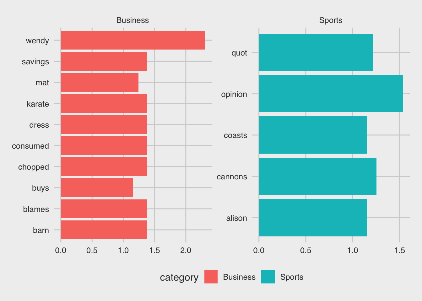
In the previous plot:
gf_colplots a barplotscales = "free"allows each plot to have independent x and y axiscoord_flipflips the corrdinates so that we get the terms on the y-axis and the tf-idf scores on the x-axis
11.5.4 Removing sparse terms
In any real text dataset, we will have thousands of unique words. So creating a document term matrix with thousands of columns might not be the best choice as it will include a lot of noise. For instance, in this data, we have 5580 distinct words:
d2 %>% distinct(word) %>% nrow## [1] 5580Let’s assume that we want to focus only on words that appear at least in 15 documents:
focal_words = d2 %>% group_by(word) %>% count() %>% filter(n > 15)
focal_words %>% nrow
## [1] 141
Note that
d2is already grouped-by document, and as a result grouping by word (see above) counts how many times each word appears in each document
We can now keep only the focal_words by running an inner join, and then, by using pivot_wider, we can get the document-term matrix:
d2 %>% inner_join(focal_words, by="word") %>%
       pivot_wider(names_from = word, values_from = tf_idf, values_fill = 0) %>%
       arrange(desc(olympics))
## # A tibble: 3,856 × 144
## title category n quot san olympics million week pay bank hurricane
## <chr> <chr> <int> <dbl> <dbl> <dbl> <dbl> <dbl> <dbl> <dbl> <dbl>
## 1 At t… Sports 22 0 0 0.635 0 0 0 0 0
## 2 Gree… Sports 22 0 0 0.347 0 0 0 0 0
## 3 Oooh… Sports 22 0 0 0.347 0 0 0 0 0
## 4 Coac… Sports 22 0 0 0.318 0 0 0 0 0
## 5 Note… Sports 22 0 0 0.318 0 0 0 0 0
## 6 Time… Sports 22 0 0 0.318 0 0 0 0 0
## 7 Aust… Sports 22 0 0 0.293 0 0 0 0 0
## 8 Judg… Sports 22 0 0 0.293 0 0 0 0 0
## 9 Nest… Sports 22 0 0 0.293 0 0 0 0 0
## 10 El G… Sports 22 0 0 0.254 0 0 0 0 0
## # … with 3,846 more rows, and 133 more variables: growth <dbl>, months <dbl>,
## # plans <dbl>, billion <dbl>, florida <dbl>, oil <dbl>, biggest <dbl>,
## # start <dbl>, night <dbl>, jobs <dbl>, sales <dbl>, games <dbl>,
## # federal <dbl>, financial <dbl>, team <dbl>, history <dbl>, london <dbl>,
## # sunday <dbl>, economic <dbl>, earnings <dbl>, report <dbl>, quarter <dbl>,
## # athens <dbl>, season <dbl>, investment <dbl>, cut <dbl>, medal <dbl>,
## # profit <dbl>, rose <dbl>, percent <dbl>, gt <dbl>, lt <dbl>, …11.5.5 Sentiment analysis
Similar to what we did in the initial example with the three documents, we can perform an inner join between our tibble and the nrc_lexicon and then aggregate to get the overall sentiment of each document in our dataset:
d1 %>%  filter(str_detect(word,"^[a-z]+$")) %>%
        inner_join(nrc_lexicon, by="word") %>%
        count(title,sentiment) %>%
        pivot_wider(names_from = sentiment, values_from = n, values_fill = 0)
## # A tibble: 960 × 11
## title negative positive sadness trust anticipation joy surprise disgust
## <chr> <int> <int> <int> <int> <int> <int> <int> <int>
## 1 "'Canes … 1 2 1 1 0 0 0 0
## 2 "'Dream … 1 5 1 2 5 3 2 0
## 3 "'I'm 10… 0 3 0 2 1 1 0 0
## 4 "'Style'… 0 3 0 2 1 2 0 0
## 5 "(17) Ut… 0 1 0 4 1 1 0 0
## 6 "\\$616m… 1 0 0 0 1 0 0 1
## 7 "#39;Can… 0 1 0 0 1 0 0 0
## 8 "#39;Pro… 3 2 1 1 1 1 0 2
## 9 "#39;Spa… 1 1 0 0 1 0 0 0
## 10 "100 win… 0 3 0 1 0 0 0 0
## # … with 950 more rows, and 2 more variables: fear <int>, anger <int>For comments, suggestions, errors, and typos, please email me at: kokkodis@bc.edu