22 Variance and standard deviation

The values of a random variable vary. The distribution of a random variable describes its pattern of variability. The expected value of a random variable summarizes the distribution in just a single number, the long run average value. But the expected value does not tell us much about the degree of variability of the random variable. Do the values of the random variable tend to be close to the expected value, or are they spread out? Variance and standard deviation are numbers that address these questions.

Example 22.1

A roulette wheel has 18 black spaces, 18 red spaces, and 2 green spaces, all the same size and each with a different number on it. Guillermo bets $1 on black. If the wheel lands on black, Guillermo wins his bet back plus an additional $1; otherwise he loses the money he bet. Let $W$ be Guillermo’s net winnings (net of the initial bet of $1.)

Find the distribution of $W$.
Compute $\text{E}(W)$.
Interpret $\text{E}(W)$ in context.
An expected profit for the casino of 5 cents per $1 bet seems small. Explain how casinos can turn such a small profit into billions of dollars.
Recall that variance is the long run average squared distance from the mean. Describe how you could use simulation to approximate the variance of $W$. What would you expect the simulation results to look like?
Without doing any further calculations, provide a ballpark estimate of the variance. Explain. What are the measurement units for the variance?
The random variable $(W-\text{E}(W))^2$ represents the squared deviation from the mean. Find the distribution of this random variable and its expected value.
Recall that standard deviation is the square root of the variance. Why would we want to take the square root of the variance? Compute and interpret the standard deviation of $W$.
Compute $\text{E}(W^2)$. (For this $W$ you should be able to compute $\text{E}(W^2)$ without any calculations; why?) Then compute $\text{E}(W^2) - (\text{E}(W))^2$; what do you notice?

The variance of a random variable $X$ is \[\begin{align*} \text{Var}(X) & = \text{E}\left(\left(X-\text{E}(X)\right)^2\right)\\ & = \text{E}\left(X^2\right) - \left(\text{E}(X)\right)^2 \end{align*}\]
The standard deviation of a random variable is \[\begin{equation*} \text{SD}(X) = \sqrt{\text{Var}(X)} \end{equation*}\]
Variance is, roughly, the long run average squared deviation from the mean.
Standard deviation measures, roughly, the long run average distance from the mean. The measurement units of the standard deviation are the same as for the random variable itself.
The definition $\text{E}((X-\text{E}(X))^2)$ represents the concept of variance. However, variance is usually computed using the following equivalent but slightly simpler formula.

\[ \text{Var}(X) = \text{E}\left(X^2\right) - \left(\text{E}\left(X\right)\right)^2 \]

That is, variance is the expected value of the square of $X$ minus the square of the expected value of $X$.
In some cases, we have the expected value and variance and we want to compute $\text{E}(X^2)$. Rearranging the above formula yields

\[ \text{E}\left(X^2\right) = \text{Var}(X) + \left(\text{E}\left(X\right)\right)^2 \]

Variance has many nice theoretical properties. Whenever you need to compute a standard deviation, first find the variance and then take the square root at the end.

Example 22.2

Continuing with roulette, Nadja bets $1 on number 7. If the wheel lands on 7, Nadja wins her bet back plus an additional $35; otherwise she loses the money she bet. Let $X$ be Nadja’s net winnings (net of the initial bet of $1.)

Find the distribution of $X$.
Compute $\text{E}(X)$.
How do the expected values of the two $1 bets — bet on black versus bet on 7 — compare? Explain what this means.
Are the two $1 bets — bet on black versus bet on 7 — identical? If not, explain why not.
Before doing any calculations, determine if $\text{SD}(X)$ is greater than, less than, or equal to $\text{SD}(W)$. Explain.
Compute $\text{Var}(W)$ and $\text{SD}(W)$.
Which $1 bet — betting on black or betting on 7 — is “riskier”? How is this reflected in the standard deviations?

Example 22.3

Let $X$ be a Uniform($a$, $b$) distribution.

First, suppose $X$ has a Uniform(0, 1) distribution. Make a ballpark estimate of the standard deviation.
Compute $\text{SD}(X)$ if $X$ has a Uniform(0, 1) distribution.
Now suggest a rough formula for the standard deviation for the general Uniform($a$, $b$) case.
Compute $\text{SD}(X)$ if $X$ has a Uniform($a$, $b$) distribution.

Example 22.4

The plots below summarize hypothetical distributions of quiz scores in six classes. All plots are on the same scale. Each quiz score is a whole number between 0 and 10 inclusive.

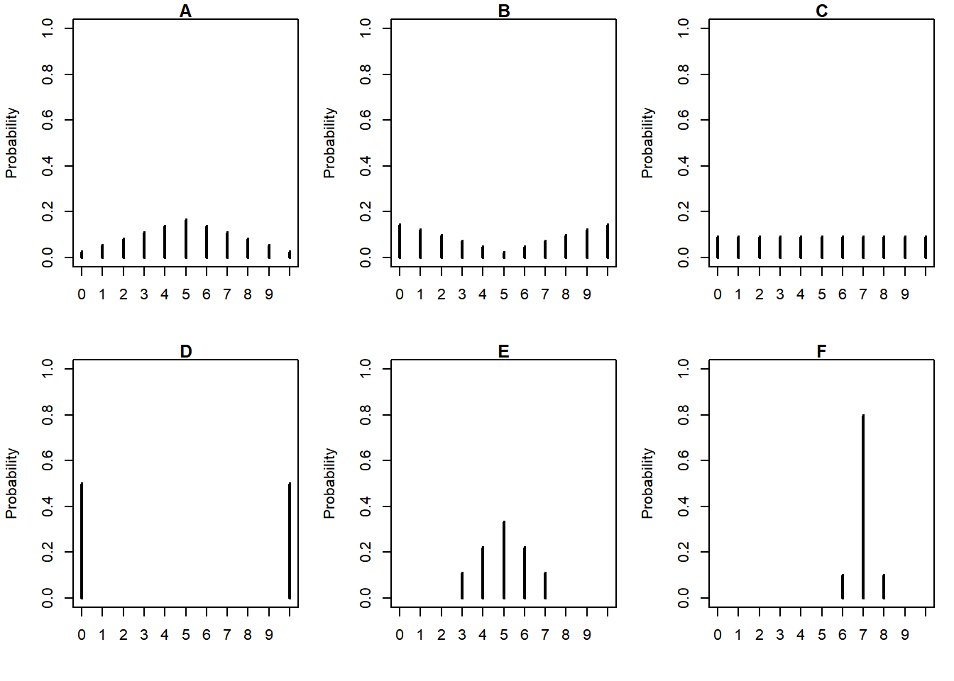
Donny Dont says that C represents the smallest SD, since there is no variability in the heights of the bars. Do you agree that C represents “no variability? Explain.
What is the smallest possible value the SD of quiz scores could be? What would need to be true about the distribution for this to happen? (This scenario might not be represented by one the plots.)
Without doing any calculations, arrange the classes in order based on their SDs from smallest to largest.
In one of the classes, the SD of quiz scores is 5. Which one? Why?
Is the SD in F greater than, less than, or equal to 1? Why?
Provide a ballpark estimate of SD in each case.

Example 22.5

Let $X$ have an Exponential(1) distribution. Make a ballpark estimate for $\text{SD}(X)$, and then compute it.

22.1 Standardization

Standard deviation provides a “ruler” by which we can judge a particular realized value of a random variable relative to the distribution of values.
If $X$ is a random variable with expected value $\text{E}(X)$ and standard deviation $\text{SD}(X)$, then the standardized random variable is

\[ Z = \frac{X - \text{E}(X)}{\text{SD}(X)} \]

However, keep in mind that comparing standardized values is most appropriate for distributions that have similar shapes.

Example 22.6

For which distribution — Uniform(0, 1) or Exponential(1) — is it more unsual to see a value smaller than 0.15?

Standardize the value 0.15 relative to the Uniform(0, 1) distribution.
Standardize the value 0.15 relative to the Exponential(1) distribution.
Donny Dont says: “For the Uniform(0, 1) distribution, a value of 0.15 is 1.2 standard deviations below the mean. For the Exponential(1) distribution, a value of 0.15 is 0.85 standard deviations below the mean. So a value smaller than 0.15 is more unusual for a Uniform(0, 1) distribution, since there it’s more standard deviations below the mean.” Do you agree with his conclusion? Explain.
How can you answer the original question in the setup?
The value 0.15 is what percentile for a Uniform(0, 1) distribution?
The value 0.15 is what percentile for an Exponential(1) distribution?
For which distribution — Uniform(0, 1) or Exponential(1) — is it more unsual to see a value smaller than 0.15?

22.2 Chebyshev’s inequality

Chebyshev’s inequality says that for any distribution, the probability that the random variable takes a value more than $z$ SDs away from its mean is at least $1 - 1 / z^2$. For any distribution,
- ($z = 2$.) At most 25% of values fall more than 2 standard deviations away from the mean.
- ($z = 3$.) At most 11.1% of values fall more than 3 standard deviations away from the mean.
- ($z = 4$.) At most 6.25% of values fall more than 4 standard deviations away from the mean.
- ($z = 5$.) At most 4% of values fall more than 5 standard deviations away from the mean.
- ($z = 6$.) At most 2.8% of values fall more than 6 standard deviations away from the mean.
- and so on, for different values of $z$.
This universal “empirical rule” works for any distribution, but will tend to be very conservative when applied to any particular distribution.
In short, Chebyshev’s inequality says that if a value is more than a few standard deviations away from the mean then it is a fairly extreme value, regardless of the shape of the distribution.