29 Normal Distributions
- Normal distributions are probably the most important distributions in probability and statistics.
- Any Normal distribution follows the “empirical rule” which determines the percentiles that give a Normal distribution its particular bell shape. For example,
- 38% of values are within 0.5 standard deviations of the mean
- 68% of values are within 1 standard deviation of the mean
- 87% of values are within 0.5 standard deviations of the mean
- 95% of values are within 2 standard deviations of the mean
- 99% of values are within 2.6 standard deviations of the mean
- 99.7% of values are within 3 standard deviations of the mean
| Percentile | SDs away from the mean |
|---|---|
| 0.1% | 3.09 SDs below the mean |
| 0.5% | 2.58 SDs below the mean |
| 1% | 2.33 SDs below the mean |
| 2.5% | 1.96 SDs below the mean |
| 10% | 1.28 SDs below the mean |
| 15.9% | 1 SDs below the mean |
| 25% | 0.67 SDs below the mean |
| 30.9% | 0.5 SDs below the mean |
| 50% | 0 SDs above the mean |
| 69.1% | 0.5 SDs above the mean |
| 75% | 0.67 SDs above the mean |
| 84.1% | 1 SDs above the mean |
| 90% | 1.28 SDs above the mean |
| 97.5% | 1.96 SDs above the mean |
| 99% | 2.33 SDs above the mean |
| 99.5% | 2.58 SDs above the mean |
| 99.9% | 3.09 SDs above the mean |
- A continuous random variable \(Z\) has a Standard Normal distribution if its pdf is \[\begin{align*} \phi(z) & = \frac{1}{\sqrt{2\pi}}\,e^{-z^2/2}, \quad -\infty<z<\infty,\\ & \propto e^{-z^2/2}, \quad -\infty<z<\infty. \end{align*}\]
- If \(Z\) has a Standard Normal distribution then \[\begin{align*} \text{E}(Z) & = 0\\ \text{SD}(Z) & = 1 \end{align*}\]
- The Standard Normal pdf is symmetric about its mean of 0, and the peak of the density occurs at 0.
- The standard deviation is 1, and 1 also indicates the distance from the mean to where the concavity of the density changes. That is, there are inflection points at \(\pm1\).
- A continuous random variable \(X\) has a Normal (a.k.a., Gaussian) distribution with mean \(\mu\in (-\infty,\infty)\) and standard deviation \(\sigma>0\) if its pdf is \[\begin{align*} f_X(x) & = \frac{1}{\sigma\sqrt{2\pi}}\,\exp\left(-\frac{1}{2}\left(\frac{x-\mu}{\sigma}\right)^2\right), \quad -\infty<x<\infty,\\ & \propto \exp\left(-\frac{1}{2}\left(\frac{x-\mu}{\sigma}\right)^2\right), \quad -\infty<x<\infty. \end{align*}\]
- If \(X\) has a Normal(\(\mu\), \(\sigma\)) distribution then \[\begin{align*} \text{E}(X) & = \mu\\ \text{SD}(X) & = \sigma \end{align*}\]
- A Normal density is a particular “bell-shaped” curve which is symmetric about its mean \(\mu\). The mean \(\mu\) is a location parameter: \(\mu\) indicates where the center and peak of the distribution is.
- The standard deviation \(\sigma\) is a scale parameter: \(\sigma\) indicates the distance from the mean to where the concavity of the density changes. That is, there are inflection points at \(\mu\pm \sigma\).
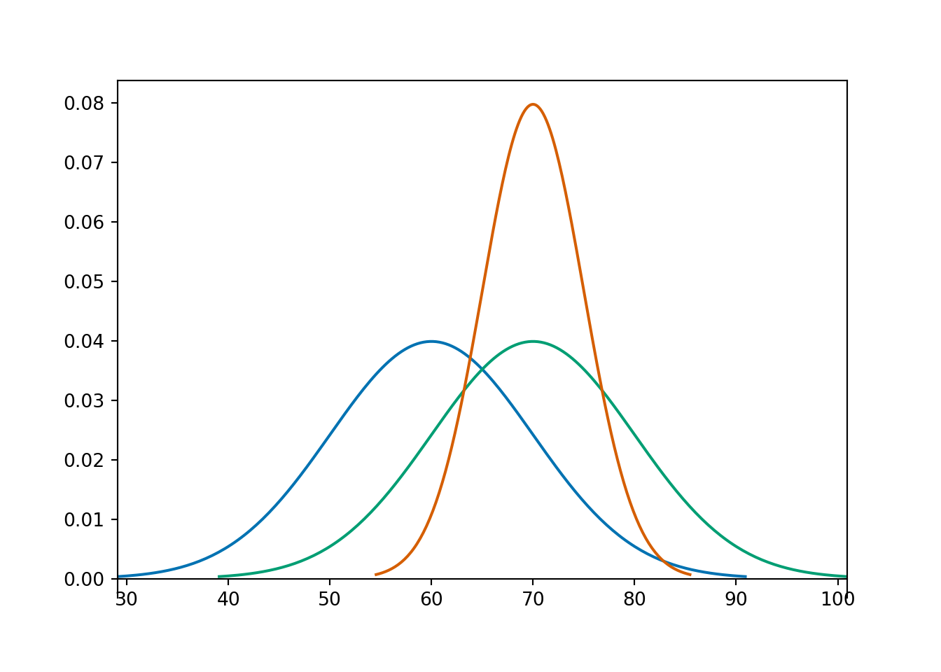
Example 29.1
The pdfs in the plot below represent the distribution of hypothetical test scores in three classes. The test scores in each class follow a Normal distribution. Identify the mean and standard deviation for each class.
Example 29.2
The wrapper of a package of candy lists a weight of 47.9 grams. Naturally, the weights of individual packages vary somewhat. Suppose package weights have an approximate Normal distribution with a mean of 49.8 grams and a standard deviation of 1.3 grams.
- Sketch the distribution of package weights. Carefully label the variable axis. It is helpful to draw two axes: one in the measurement units of the variable, and one in standardized units.
- Why wouldn’t the company print the mean weight of 49.8 grams as the weight on the package?
- Estimate the probability that a package weighs less than the printed weight of 47.9 grams.
- Estimate the probability that a package weighs between 47.9 and 53.0 grams.
- Suppose that the company only wants 1% of packages to be underweight. Find the weight that must be printed on the packages.
- Find the 25th percentile (a.k.a., first (lower) quartile) of package weights.
- Find the 75th percentile (a.k.a., third (upper) quartile) of package weights. How can you use the work you did in the previous part?
Example 29.3
Daily high temperatures (degrees Fahrenheit) in San Luis Obispo in August follow (approximately) A Normal distribution with a mean of 76.9 degrees F. The temperature exceeds 100 degrees Fahrenheit on about 1.5% of August days.
- What is the standard deviation?
- Suppose the mean increases by 2 degrees Fahrenheit. On what percentage of August days will the daily high temperature exceed 100 degrees Fahrenheit? (Assume the standard deviation does not change.)
- A mean of 78.9 is 1.02 times greater than a mean of 76.9. By what (multiplicative) factor has the percentage of 100-degree days increased? What do you notice?
Example 29.4 In a large class, scores on midterm 1 follow (approximately) a Normal\((\mu_1, \sigma)\) distribution and scores on midterm 2 follow (approximately) a Normal\((\mu_2, \sigma)\) distribution. Note that the SD \(\sigma\) is the same on both exams. The 40th percentile of midterm 1 scores is equal to the 70th percentile of midterm 2 scores. Compute
\[ \frac{\mu_1-\mu_2}{\sigma} \]
(This is one statistical measure of effect size.)
- If \(X\) and \(Y\) are independent, each with a marginal Normal distribution, and \(a, b\) are non-random constants then \(aX + bY\) has a Normal distribution.
Example 29.5
Two people are meeting. (Who? You decide!) Arrival time are measured in minutes after noon, with negative times representing arrivals before noon. Each arrival time follows a Normal distribution with mean 30 and SD 17 minutes, independently of each other.
- Compute the probability that the first person to arrive has to wait more than 15 minutes for the second person to arrive.
- Compute the probability that the first person to arrive arrives before 12:15.