Chapter 13 Date and time series
시계열 자료를 분석을 위해 필요한 부분은 날짜에 대한 데이터 변환입니다. 보통의 데이터가 오류를 없애기 위해 날짜를 문자나 숫자로 입력합니다. 이를 날짜 변수로 변환하는 과정을 실습하도록 하겠습니다. 엑셀과 SAS, R은 숫자로 변환된 날짜를 다시 날짜로 변환할 때 기준점이 다릅니다. 그렇게 때문에 주의가 필요합니다.
필요한 라이브러리를 불러 오겠습니다.
rm(list=ls())
Sys.setenv(LANG = "en")
library(tidyverse)
library(lubridate)
library(data.table)
library(dplyr)
#library(doMC)
#registerDoMC(47)
library(htmlTable)
library(gam)본 자료는 실제 자료를 기반으로 가상의 랜덤 값을 준 것 입니다. 가상의 자료이니 본 분석 결과를 사실로 받아 들이시지는 마시기 바랍니다.
## [1] "date" "temp_mean" "temp_max" "cloud_mean" "sun_day"
## [6] "wind_mean" "rhum_mean" "temp" "tempf" "humidity"
## [11] "heat_index" "event" "period" "region_id" "inclusion"
## [16] "year" "circulation" "cvd" "endo" "gi"
## [21] "heat" "infection" "injury" "mental" "nmd"
## [26] "respiratory" "skin" "uro" "tmr" "occp1"
## [31] "occp2" "occp3" "occp4" "occp5" "occp6"
## [36] "occp7" "occp8" "occp9" "occp13" "occp99"
## [41] "inside" "outside" "tomr"13.1 Date create
오늘 날짜와 지금 시간, 초를 생성해 보겠습니다. 어떻게 나오나요?
주로 날짜는 엑셀 등으로 저잘할 때 문자형식으로 저장합니다. 숫자로 저장하는 경우 변환할때 한번더 수작업을 해야 하기 때문입니다. 또한 월이 있는데, 일이 없거나 하는 경우 변환때 missing 값을로 자동변환됨에도 연구자가 모르고 지나 갈수 있기 때문입니다. 문자로 저장된 날짜를 날짜 변수로 만들어 보겠습니다.
ymd, mdy, dmy를 사용하겠습니다.
tibble(ymd("2020-11-10"),
ymd("20201110"),
ymd("2020-Nov-10"),
mdy("November 10th, 2020"),
dmy("10-Nov-2020")) %>% t() ## [,1]
## ymd("2020-11-10") "2020-11-10"
## ymd("20201110") "2020-11-10"
## ymd("2020-Nov-10") "2020-11-10"
## mdy("November 10th, 2020") "2020-11-10"
## dmy("10-Nov-2020") "2020-11-10"모든 날짜는 숫자로 저장되고 있습니다. 2020년 11월 10일은 숫자로는 18576입니다. 기준 날짜인 1970년 1월 1일부터 몇일이 지났는지를 적어 놓은 것입니다. 그래서 아래의 함수를 통해 숫자를 날짜로 변환 할 수 있습니다.
## [1] 18576## [1] "2020-11-10"2020년 11월 10일부터 100일이 지난 날의 날짜는 무엇일까요? 아래와 같이 해볼 수 있습니다.
## [1] "2021-02-18"여기에 hour, minute, second를 추가할 수 있습니다 .
tibble(year = 2020,
month = 11,
day = 10,
hour = 11,
minute= 15,
sec = 30) %>%
mutate(now = make_datetime(
year, month, day, hour, minute, sec
)) ## # A tibble: 1 x 7
## year month day hour minute sec now
## <dbl> <dbl> <dbl> <dbl> <dbl> <dbl> <dttm>
## 1 2020 11 10 11 15 30 2020-11-10 11:15:30그럼 그냥 문자로 사용하면 되지 왜 date 형식으로 변환을 하는 걸까요? Date-time components 가 필요하기 때문이기도 합니다. 그리고 연산이 가능해 집니다.
## [1] 2020## [1] 11## [1] 10## [1] 315## [1] 3몇월인지 무슨 요일인지 생성해 보겠습니다.
## [1] 11월
## 12 Levels: 1월 < 2월 < 3월 < 4월 < 5월 < 6월 < 7월 < 8월 < ... < 12월## [1] 화
## Levels: 일 < 월 < 화 < 수 < 목 < 금 < 토13.2 Tutor: heat wave and death
hm0 자료를 가지고 몇가지 실습을 해보도록 하겠습니다.
## date temp_mean temp_max cloud_mean sun_day wind_mean rhum_mean temp
## 1: 2002-01-01 -4.4222222 4.6 1.6333333 7.577778 2.966667 55.62222 -1.5
## 2: 2002-01-02 -11.6222222 -4.7 0.1777778 8.033333 3.566667 40.97778 -8.7
## 3: 2002-01-03 -8.2222222 1.9 1.3111111 8.011111 3.266667 45.83333 -3.6
## 4: 2002-01-04 0.3777778 7.6 5.9666667 2.811111 3.800000 66.02222 2.7
## 5: 2002-01-05 -2.6777778 4.0 0.5333333 7.855556 2.833333 45.53333 0.5
## 6: 2002-01-06 -3.6222222 8.4 1.2333333 8.055556 1.477778 54.55556 1.2
## tempf humidity heat_index event period region_id inclusion year circulation
## 1: 29.3 44.5 -1.51 0 0 42 1 2002 0
## 2: 16.4 27.1 -8.69 0 0 42 1 2002 10
## 3: 25.6 24.1 -3.58 0 0 42 1 2002 10
## 4: 36.8 47.9 2.68 0 0 42 1 2002 16
## 5: 32.8 29.4 0.45 0 0 42 1 2002 8
## 6: 34.2 32.4 1.23 0 0 42 1 2002 0
## cvd endo gi heat infection injury mental nmd respiratory skin uro tmr occp1
## 1: 0 0 0 0 0 0 0 0 0 0 0 27 0
## 2: 0 1 23 0 5 6 6 26 76 10 17 27 0
## 3: 1 7 10 0 8 8 2 12 63 10 12 25 0
## 4: 1 7 12 0 5 4 2 17 57 16 12 29 0
## 5: 0 1 13 0 1 7 1 16 36 8 5 25 0
## 6: 0 0 0 0 0 0 0 0 0 0 0 23 1
## occp2 occp3 occp4 occp5 occp6 occp7 occp8 occp9 occp13 occp99 inside outside
## 1: 0 0 0 2 3 0 0 0 22 0 27 0
## 2: 0 1 0 3 3 1 0 1 18 0 27 0
## 3: 0 0 1 0 6 0 0 0 18 0 25 0
## 4: 0 0 1 4 3 2 0 1 18 0 29 0
## 5: 1 0 1 1 4 0 0 0 18 0 25 0
## 6: 0 0 0 0 5 1 0 0 16 0 23 0
## tomr
## 1: 5
## 2: 9
## 3: 7
## 4: 11
## 5: 7
## 6: 713.2.1 date create
날짜를 생성해 보겠습니다.
## [1] "Date"## [1] "numeric"2002년부터 2015년까지의 자료 입니다.
## # A tibble: 14 x 2
## # Groups: year [14]
## year n
## <dbl> <int>
## 1 2002 24820
## 2 2003 24820
## 3 2004 24892
## 4 2005 24824
## 5 2006 24824
## 6 2007 24835
## 7 2008 24894
## 8 2009 24822
## 9 2010 24856
## 10 2011 25200
## 11 2012 25267
## 12 2013 25220
## 13 2014 25213
## 14 2015 25212월, 일, 숫자형 월을 생성해 보겠습니다.
s2 <- hm0 %>% mutate(months = lubridate::month(date, label = TRUE, abbr = TRUE)) %>%
mutate(weekday = lubridate::wday(date, label = TRUE, abbr = TRUE)) %>%
mutate(month = substr(date, 6, 7)) %>%
filter(year(date) <= 2015) 월별 햇볕이 있었던 날의 수를 표로 나타내 보겠습니다.
s2 %>% group_by(months) %>%
summarize(`number of sunny days` = sum(sun_day, na.rm=TRUE)) %>%
htmlTable()| months | number of sunny days | |
|---|---|---|
| 1 | 1월 | 163634.1 |
| 2 | 2월 | 160058 |
| 3 | 3월 | 196690 |
| 4 | 4월 | 196703.6 |
| 5 | 5월 | 216350.7 |
| 6 | 6월 | 173973.8 |
| 7 | 7월 | 132143 |
| 8 | 8월 | 154961.4 |
| 9 | 9월 | 160004.7 |
| 10 | 10월 | 197543.7 |
| 11 | 11월 | 150447.1 |
| 12 | 12월 | 153073.2 |
월별 분포를 그림으로 그려보겠습니다.
library(ggplot2)
s2 %>% filter(year ==2015) %>%
group_by(months) %>%
ggplot(aes(x= months, y = sun_day, color = months)) +
geom_point()+
ggtitle('sunny day counts by months') +
ylab ('sunny day counts') +
guides(color = FALSE) 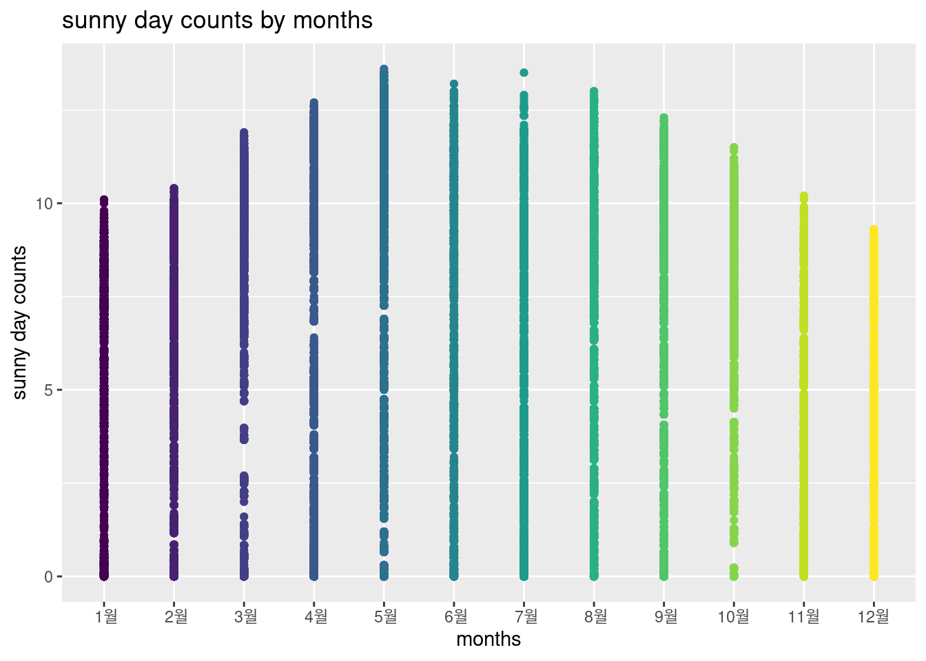
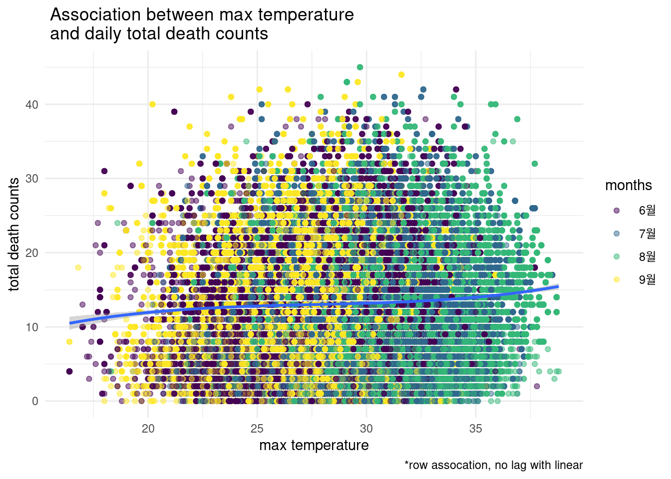
이번에는 최고 기온가 일병 사망 숫자와의 관계를 살폐보겠습니다. 고온과 사망이므로 filter(month %in% c("06", "07", "08", "09"))을 이용하겠습니다. 월을 만들어 놓았으니 filter를 이용해서 필요한 월만 가져오면 되겠습니다. tomr 은 total occupation mortality 입니다. count 입니다. 35도가 넘으면 사망 숫자가 상승하고 있습니다.
s2 %>% filter(month %in% c("06", "07", "08", "09"),
temp_max >15) %>%
ggplot(aes(x = lag(temp_max), y = tomr)) +
geom_point(aes(color = months), alpha = 0.5) +
stat_smooth(method = "lm", formula = y ~ poly(x, 3), size = 1) +
theme_minimal() +
xlab('max temperature') + ylab('total death counts') +
labs(caption ="*row assocation, no lag with linear",
title=" Association between max temperature \n and daily total death counts "#, subtitle="Beta = -0.014, p = 0.158 before 2009\n Beta = 0.002, p = 0.011 from 2009"
)
13.3 home work
13.3.1 home0
2020-11-10로부터 100일전 날짜는?
2020-11-10로 부터 100일전 날짜의 요일은?
1978-01-21 에 태어난 사람이 2020-12-31까지 몇일을 살았을까?
1919-03-01 은 무슨 요일일까?
13.3.2 home work1
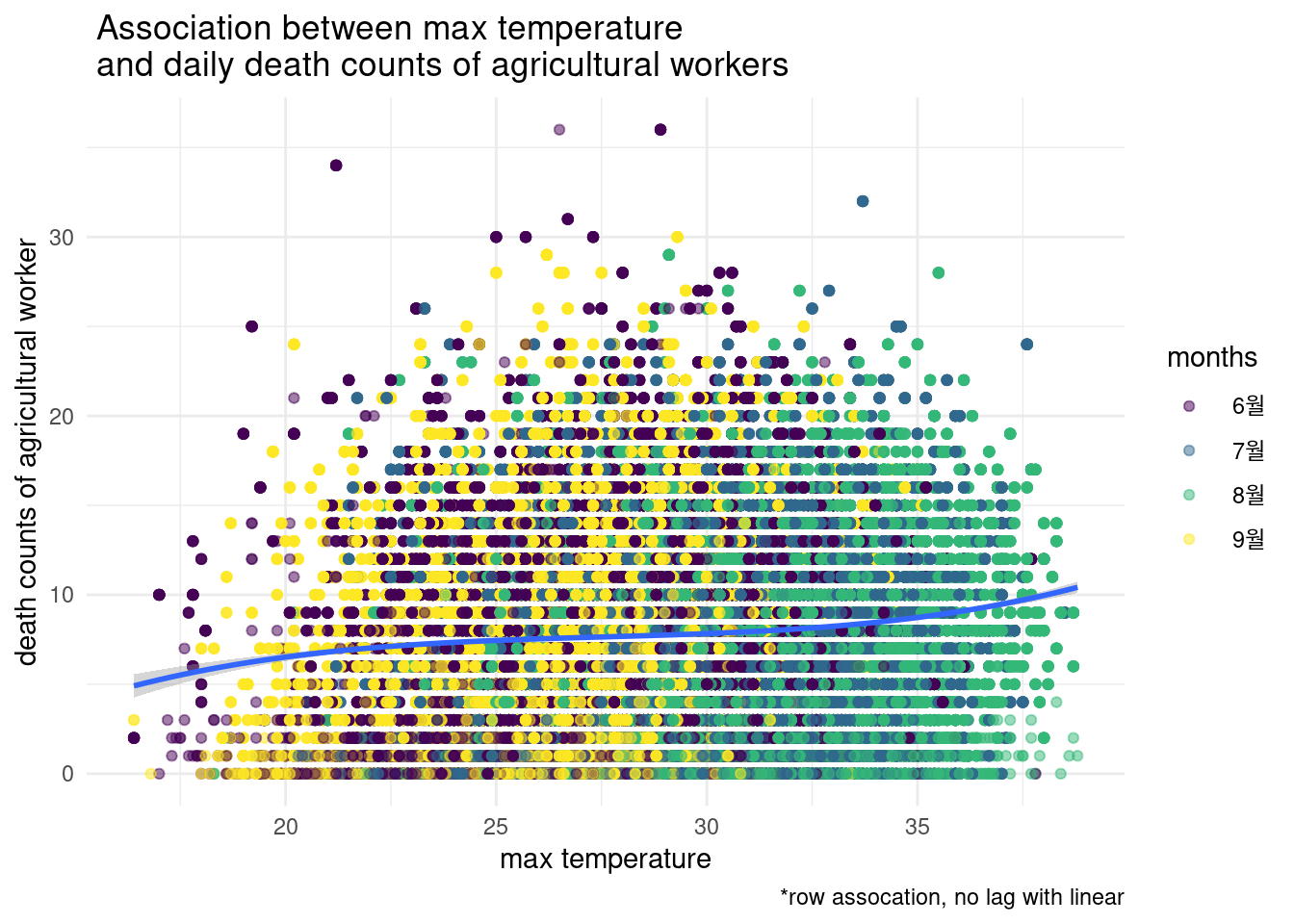
6, 7, 8, 9월에 고온과 농업인의 사망과의 관련성을 그려보세요. 농업인의 사망은 occp6 입니다.
13.3.3 home work2
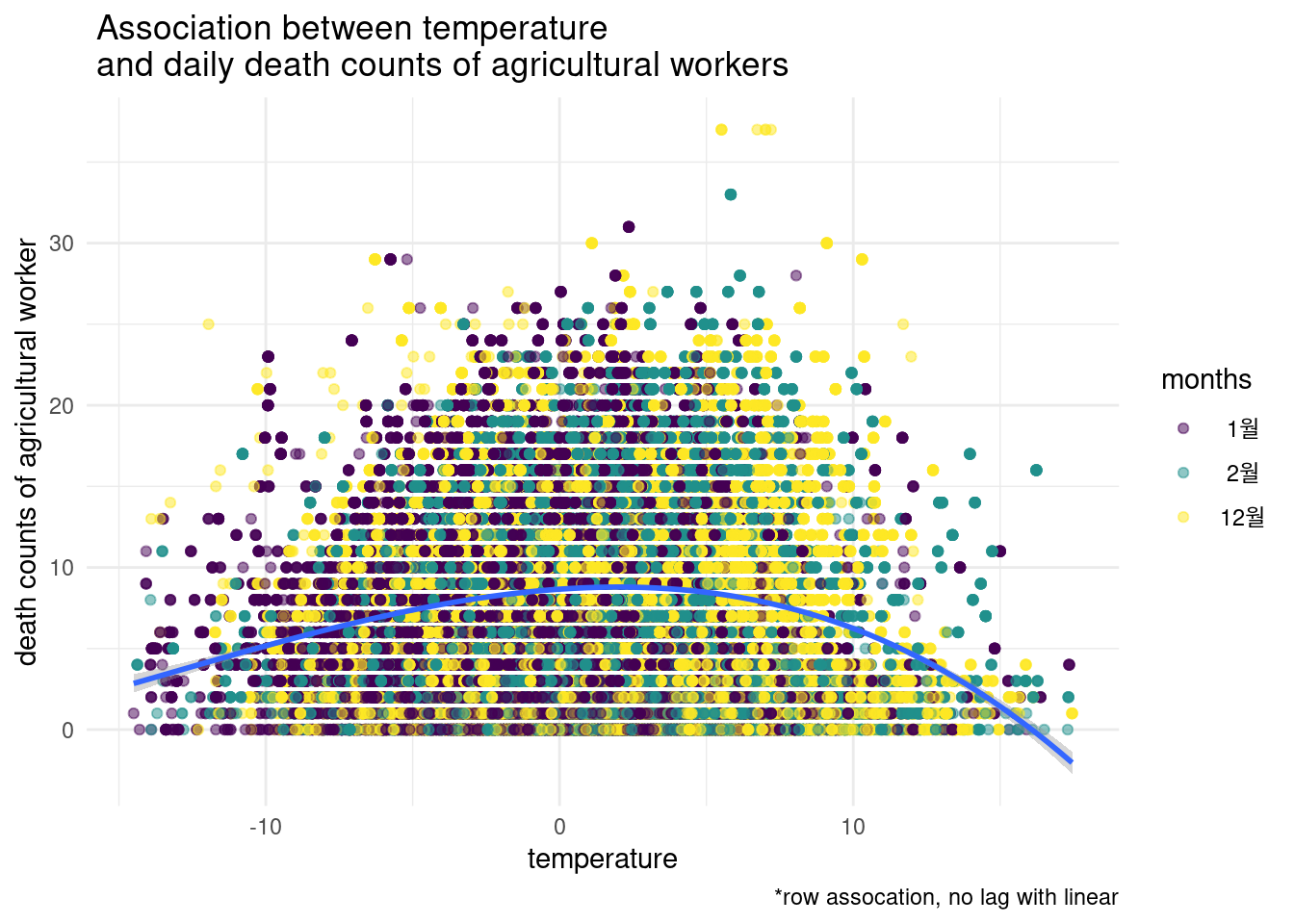
12, 1, 2월에 기온과 농업인의 사망과의 관련성을 그려보세요. 기온은 temp_mean을 농업인의 사망은 occp6 입니다.
13.3.4 home work3
12, 1, 2월에 기온과 관리직의 사망과의 관련성을 그려보세요. 기온은 temp_mean을 관리직의 사망은 occp1 입니다.
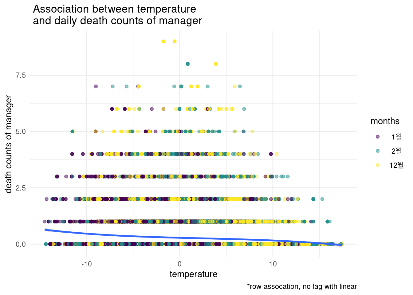
13.4 Time series data analysis
기온등의 시계열적 변수가 질병에 어떻게 영향을 미치는지 알고자 할 때 어떻게 해야 할 까요? 우선 전체 직업군의 사망수 ’tomr’을 타겟 변수로 지정하겠습니다. 그리고 월별 사망률을 그려보겠습니다.
##
## Attaching package: 'plotly'## The following object is masked from 'package:ggplot2':
##
## last_plot## The following object is masked from 'package:stats':
##
## filter## The following object is masked from 'package:graphics':
##
## layouts2 %>% group_by(months) %>%
plot_ly( x= ~ months, y = ~dz,
type = "box",
color = ~ months) %>%
layout(title = 'daily total mortality counts by months',
yaxis = list(title ='daily death counts'))## Warning: `arrange_()` is deprecated as of dplyr 0.7.0.
## Please use `arrange()` instead.
## See vignette('programming') for more help
## This warning is displayed once every 8 hours.
## Call `lifecycle::last_warnings()` to see where this warning was generated.월별 사망수의 차이가 관찰되고 있습니다. 이번에는 주별 차이를 관찰해 보겠습니다.
s2 %>% group_by(weekday) %>%
plot_ly( x= ~ weekday, y = ~dz,
type = "box",
color = ~ weekday) %>%
layout(title = 'daily total mortality counts by weekdays',
yaxis = list(title ='daily mortality counts'))고온에 대해서 알아보기 위해 6월부터 9월까지의 데이터로만 해보겠습니다. 몇다 방정식으로 모델을 구성했는지 관찰해 보세요
s2 %>% filter(month %in% c("06", "07", "08", "09"),
temp_max >15) %>%
ggplot(aes(x = lag(temp_max, 2), y = dz)) +
geom_point(aes(color = months), alpha = 0.5) +
stat_smooth(method = "lm", formula = y ~ poly(x, 3), size = 1) +
theme_minimal() +
xlab('max temperature') + ylab('total death counts') +
labs(caption ="*row assocation, no lab with linear",
title=" Association between max temperature \n and daily total death counts ")## Warning: Removed 2 rows containing non-finite values (stat_smooth).## Warning: Removed 2 rows containing missing values (geom_point).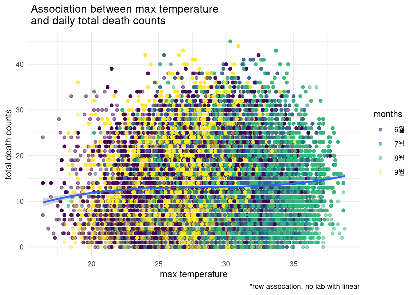
기본적인 분석을 시행해 보겠습니다. 단순 회귀분석을 시행한다고 생각하고 진행해 보겠습니다. glm을 이용해 모델을 만들고, summary()를 통해 통계 값을 구해보겠습니다.
s2 <- s2%>% mutate(index = row_number())
mod1 <- glm(data = s2,
dz ~ temp_max + weekday + months + ns(index) +
region_id, family = quasipoisson())
summary(mod1)$coefficient[1,]## Estimate Std. Error t value Pr(>|t|)
## 2.494459e+00 4.660113e-03 5.352786e+02 0.000000e+00위에서 무엇이 단순 회귀 분서과 시계열 분석의 차이가 될까요? ns(index) 부분이 될 것입니다. 좀더 자세히 보겠습니다. 아래는 최고 온도의 변호와 3일의 간격을 두고, 주말 효과는 자유도 6으로 각 주가 각기 다른 효과를 준다고 가정하고, 월은 월을 dummy 변수로 취급하고, index에는 10을 주어서 시계열적 변화를 보정한다 이런 뜻 정도로 이해할 수 있습니다. 여기서 각 3, 6, 10 등의 숫자를 무엇을 넣어야 할지가 시계열 분석에서 고민해야 할 지점 중 하나입니다. 이는 다음 시간에 simulation하는 과정을 통해 알아보고 우선 진행해 보겠습니다.
g.mod1 <- glm(data = s2,
dz ~ lag(temp_max, 3) +
ns(week(date), 6) +
as.factor(months) +
ns(index, 10) + region_id, family = quasipoisson())
summary(g.mod1)$coefficient## Estimate Std. Error t value Pr(>|t|)
## (Intercept) 2.689605306 2.030906e-02 132.4337587 0.000000e+00
## lag(temp_max, 3) 0.008380698 2.140835e-04 39.1468619 0.000000e+00
## ns(week(date), 6)1 -0.119623009 2.338702e-02 -5.1149320 3.140191e-07
## ns(week(date), 6)2 -0.253319594 2.683492e-02 -9.4399234 3.752232e-21
## ns(week(date), 6)3 -0.271267053 3.052486e-02 -8.8867588 6.320564e-19
## ns(week(date), 6)4 -0.108926422 3.202452e-02 -3.4013445 6.706277e-04
## ns(week(date), 6)5 -0.085539954 3.986917e-02 -2.1455163 3.191228e-02
## ns(week(date), 6)6 -0.011664855 3.283241e-02 -0.3552848 7.223765e-01
## as.factor(months).L 0.035538490 3.812434e-02 0.9321732 3.512477e-01
## as.factor(months).Q 0.011562176 1.835534e-02 0.6299081 5.287552e-01
## as.factor(months).C -0.005909232 1.247490e-02 -0.4736896 6.357216e-01
## as.factor(months)^4 -0.028358118 9.514330e-03 -2.9805690 2.877332e-03
## as.factor(months)^5 -0.007483562 8.059884e-03 -0.9284950 3.531515e-01
## as.factor(months)^6 -0.001183933 6.422780e-03 -0.1843334 8.537520e-01
## as.factor(months)^7 0.003316206 3.614635e-03 0.9174389 3.589134e-01
## as.factor(months)^8 0.012798534 4.307070e-03 2.9715178 2.963519e-03
## as.factor(months)^9 -0.003655662 2.963199e-03 -1.2336878 2.173201e-01
## as.factor(months)^10 -0.001302690 3.038167e-03 -0.4287750 6.680873e-01
## as.factor(months)^11 0.003369847 2.982248e-03 1.1299686 2.584902e-01
## ns(index, 10)1 -0.058476904 6.546277e-03 -8.9328495 4.171157e-19
## ns(index, 10)2 -0.057460708 8.608243e-03 -6.6750798 2.474642e-11
## ns(index, 10)3 -0.220889502 7.787630e-03 -28.3641496 8.900638e-177
## ns(index, 10)4 -0.093998725 8.275388e-03 -11.3588293 6.785182e-30
## ns(index, 10)5 -0.114886433 7.986495e-03 -14.3850886 6.621038e-47
## ns(index, 10)6 -0.140188072 8.105597e-03 -17.2952194 5.450567e-67
## ns(index, 10)7 -0.013922461 7.906394e-03 -1.7609118 7.825421e-02
## ns(index, 10)8 -0.167982193 6.611226e-03 -25.4086293 2.729150e-142
## ns(index, 10)9 0.154066429 1.314857e-02 11.7173555 1.052933e-31
## ns(index, 10)10 -0.038049443 5.825723e-03 -6.5312827 6.529763e-11
## region_id -0.000312727 1.516356e-06 -206.2358381 0.000000e+0013.4.1 outside 사망에 대해서
몇가지를 탐색해보니, 여름철 야외 사망에 대해 연구해 보면 좋겠다는 생각이 드네요.
s3 <- s2 %>%
# filter(region_id %in%c(46)) %>%
filter(month %in% c( '07', '08', '09')) %>%
mutate(index = row_number()) 위에서 얼마의 lag time을 주어야 할지 시물레이션을 돌리는 방법을 생각했었습니다. 한 방법은 가능한한 모든 것을 다 해보고 가장 적당하다고 생각되는 것을 해보는 것입니다.
## This is dlnm 2.4.2. For details: help(dlnm) and vignette('dlnmOverview').cb1<- crossbasis(s3$temp_max, lag=14, argvar=list("lin"), arglag = list(fun="poly", degree=3))
model1<-glm(data=s3,
outside ~ cb1 + weekday + months + ns(index,10) + as.factor(region_id)#+
#cloud_mean + sun_day #+ wind_mean + rhum_mean
, family=quasipoisson())
summary(model1)##
## Call:
## glm(formula = outside ~ cb1 + weekday + months + ns(index, 10) +
## as.factor(region_id), family = quasipoisson(), data = s3)
##
## Deviance Residuals:
## Min 1Q Median 3Q Max
## -3.7374 -0.9769 -0.0906 0.4888 6.1393
##
## Coefficients:
## Estimate Std. Error t value Pr(>|t|)
## (Intercept) -5.820e+01 8.141e-01 -71.488 < 2e-16 ***
## cb1v1.l1 1.096e-02 5.851e-04 18.726 < 2e-16 ***
## cb1v1.l2 -7.797e-02 5.881e-03 -13.259 < 2e-16 ***
## cb1v1.l3 1.470e-01 1.408e-02 10.441 < 2e-16 ***
## cb1v1.l4 -8.375e-02 9.276e-03 -9.029 < 2e-16 ***
## weekday.L -5.868e-03 6.136e-03 -0.956 0.338954
## weekday.Q 2.371e-02 6.155e-03 3.853 0.000117 ***
## weekday.C 2.768e-02 6.144e-03 4.506 6.61e-06 ***
## weekday^4 -8.264e-03 6.164e-03 -1.341 0.180078
## weekday^5 1.279e-03 6.155e-03 0.208 0.835338
## weekday^6 1.140e-02 6.188e-03 1.842 0.065418 .
## months.L 2.777e-02 4.420e-03 6.283 3.34e-10 ***
## months.Q -2.379e-02 5.404e-03 -4.403 1.07e-05 ***
## ns(index, 10)1 6.024e+01 8.031e-01 75.009 < 2e-16 ***
## ns(index, 10)2 6.128e+01 8.204e-01 74.693 < 2e-16 ***
## ns(index, 10)3 6.041e+01 8.124e-01 74.368 < 2e-16 ***
## ns(index, 10)4 6.133e+01 8.170e-01 75.063 < 2e-16 ***
## ns(index, 10)5 5.921e+01 8.139e-01 72.748 < 2e-16 ***
## ns(index, 10)6 5.872e+01 8.165e-01 71.918 < 2e-16 ***
## ns(index, 10)7 5.921e+01 8.152e-01 72.634 < 2e-16 ***
## ns(index, 10)8 4.090e+01 5.737e-01 71.284 < 2e-16 ***
## ns(index, 10)9 1.123e+02 1.543e+00 72.776 < 2e-16 ***
## ns(index, 10)10 2.327e+01 3.315e-01 70.180 < 2e-16 ***
## as.factor(region_id)26 -1.671e+00 2.638e-02 -63.357 < 2e-16 ***
## as.factor(region_id)27 -1.448e+00 2.412e-02 -60.036 < 2e-16 ***
## as.factor(region_id)28 -1.501e+00 1.914e-02 -78.429 < 2e-16 ***
## as.factor(region_id)29 -2.247e+00 3.379e-02 -66.487 < 2e-16 ***
## as.factor(region_id)30 -1.984e+00 3.032e-02 -65.452 < 2e-16 ***
## as.factor(region_id)31 -2.744e+00 4.254e-02 -64.510 < 2e-16 ***
## as.factor(region_id)41 3.948e-02 1.198e-02 3.297 0.000978 ***
## as.factor(region_id)42 -1.624e+00 1.352e-02 -120.127 < 2e-16 ***
## as.factor(region_id)43 -1.776e+00 1.674e-02 -106.135 < 2e-16 ***
## as.factor(region_id)44 -1.388e+00 1.448e-02 -95.896 < 2e-16 ***
## as.factor(region_id)45 -1.726e+00 1.455e-02 -118.582 < 2e-16 ***
## as.factor(region_id)46 -1.445e+00 1.366e-02 -105.782 < 2e-16 ***
## as.factor(region_id)47 -8.196e-01 1.206e-02 -67.970 < 2e-16 ***
## as.factor(region_id)48 -1.236e+00 1.301e-02 -94.956 < 2e-16 ***
## as.factor(region_id)4950 -2.781e+00 2.364e-02 -117.630 < 2e-16 ***
## ---
## Signif. codes: 0 '***' 0.001 '**' 0.01 '*' 0.05 '.' 0.1 ' ' 1
##
## (Dispersion parameter for quasipoisson family taken to be 1.109338)
##
## Null deviance: 363575 on 88109 degrees of freedom
## Residual deviance: 97171 on 88072 degrees of freedom
## (14 observations deleted due to missingness)
## AIC: NA
##
## Number of Fisher Scoring iterations: 9pred1.cb1 <-crosspred(cb1, model1, at=1:100, bylag=0.1, cumul=FALSE)
plot(pred1.cb1, "slices", var=1, col=3, ylab="Relative risk of total death count", #ci.arg=list(density=50, lwd=1),#
main="Temporal effect of max temperature on total death count",
ci.arg=list(density=100, lwd=3),
cex.main =1.5,
xlab="Lag (days)", # family="A",#ylim=c(0.980, 1.02),
col='black') ;grid()
title(main="* by 1 unit increments of max temperature",
family="A",
adj=1, line=0, font.main=1, cex=1)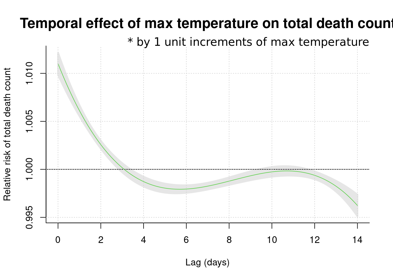
dlnm distribute lag liner and non-linear model 의 약자로 자세한 것은 http://www.ag-myresearch.com/package-dlnm.html 을 찾아 보시기 바랍니다.
여기서 주목할 점은 14일까지의 lag time을 모두 그려서 lag time이 0 인 날 즉 최고 온도가 높은 날 바로 당이에 사망이 높게 올라간다는 것입니다. 이후 4일 후에는 havesting effect가 보이는 군요. 따라서 lag time은 0 설정하고 위험도를 산출하는 방법을 사용하면 좋을 것 같습니다. 또는 그림 그대로를 받아 들여도 좋습니다.
13.5 Time series data analysis, regression
13.6 introduction
시계열적 자료를 분석하고 나타나는 현상과 특정 요인과 관련성을 탐색해보는 시간입니다.
예를 들어 미세먼지가 높은 날 심혈관 질환이 발생하는가?에 대한 질문에 답하기 위해서 생가할 것이 몇가지 있습니다.
미세먼지가 높은 날이란? 심혈관 질환 사망이 높은 날이란? 이 두가지 요소를 검토하게 됩니다.
그런데 심혈관 질환의 사망은 요일마다 다르고, 계절에 따라 변동하며, 장기 적으로는 점차 증가 또는 감소를 합니다. 그런데 미세먼지도 점차 증가하고 있으니, 단순 상관관계를 보면 미세먼지도 증가 심혈관 사망도 증가하면 양의 관련성을 보이게 됩니다.
GDP와 자살의 관계를 보면 어떨까요? 우리나라의 자살률은 증가하고 있습니다. 그런데 GDP도 증가하고 있습니다. 그러니 GDP의 증가와 자살의 증가는 양의 상관관계가 있다고 나옵니다. 맞나요?
네 심혈관 사망, 자살의 증가의 계절적 요소, 장기간 추세(trend)가 아니라 변동이 미세먼지나 GDP의 변동가 어떠한 관계가 있는지가 우리의 궁금증일 것 입니다. 이러한 궁금증을 R을 이용해서 풀어보도록 하겠습니다.
13.7 미세먼지와 심혈관사망
우선 몇가지 시계열 자료 분석의 이해를 돕기 위해 시뮬레이션 자료를 이용해 보겠습니다.
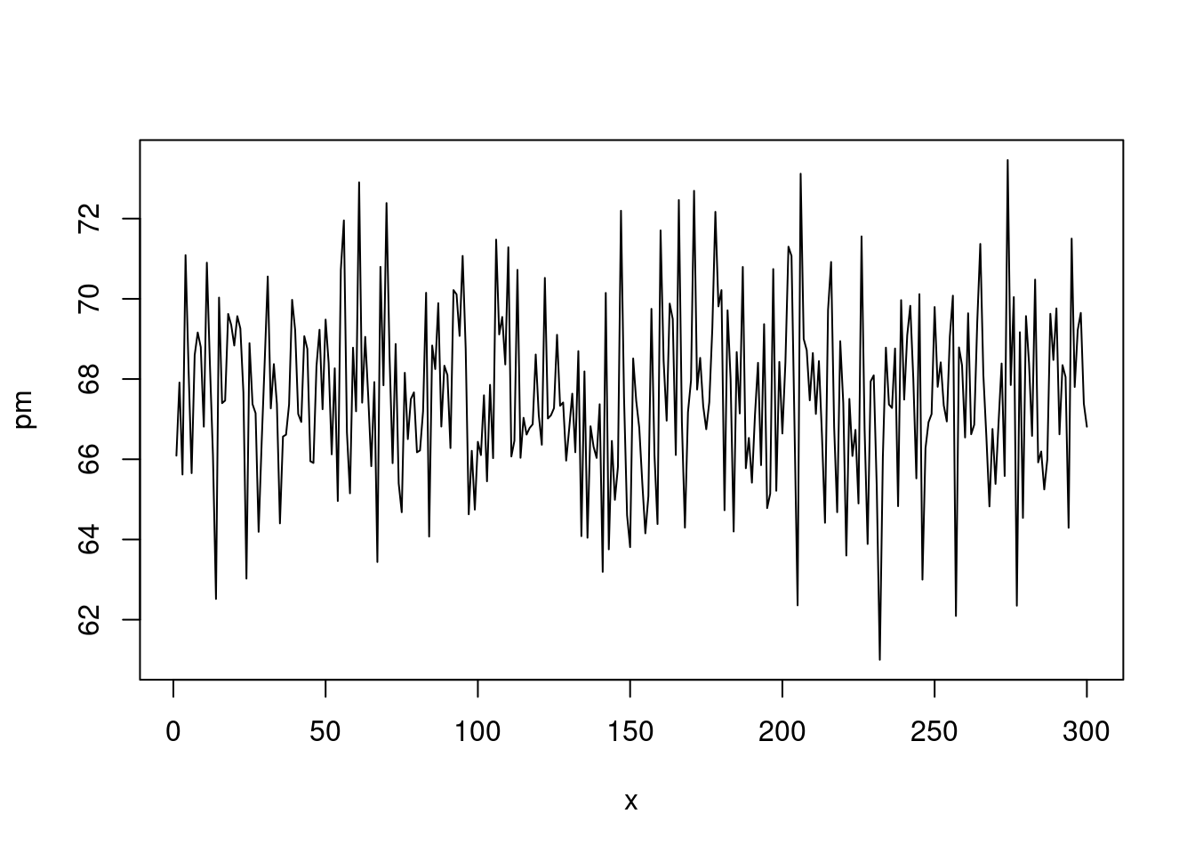
x를 일(day) 로 생각하고, 300일 동안 랜덤 변수 y1과 이에 4.5를 곱한 pm(미세먼지)를 가상으로 만들어 보겠습니다.
여기에
sin()함수를 통해 계절적 요소를 넣고, 0.03을 곱해 long term trend 가 서서히 증가하는 것으로 가정했습니다.
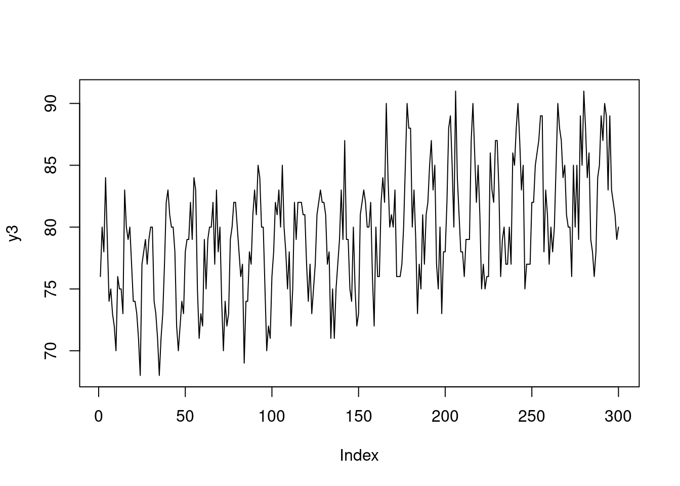
지연 효과와 특정 이벤트가 있는 날을 넣어 보았습니다. 그리고 dataframe을 만들었습니다.
## [1] 79.58667death <- c(rep(c(80,79,81), (lag/3)), y3[1:(length(y3)-lag)])
event <- c(rep(1, 30), rep(1, 30), rep(0, 240))
eventd <- c(rep(40,30), rep(30, 30), rep(0, 240))
death2<-death+eventd+10
gg <- data.frame(x, pm, y3, death, event, death2)
head(gg)## x pm y3 death event death2
## 1 1 66.09048 76 80 1 130
## 2 2 67.91320 80 79 1 129
## 3 3 65.61984 78 81 1 131
## 4 4 71.08938 84 80 1 130
## 5 5 68.24139 79 79 1 129
## 6 6 65.65395 74 81 1 131이제 그림을 그려 보겠습니다. 첫 50일에 이벤트가 있어 심혈관 사망이 높고 이후 계절적 요소를 보이며 서서히 증가하고 있습니다. 미세먼지는 random + 계절적 요소로 만들었고요.
plot(x, pm, type="l", col=grey(0.5), ylim=c(50, 140), xlim=c(0, 300))
grid()
lines(x, death2, col=grey(0.7), type="p", cex=0.5)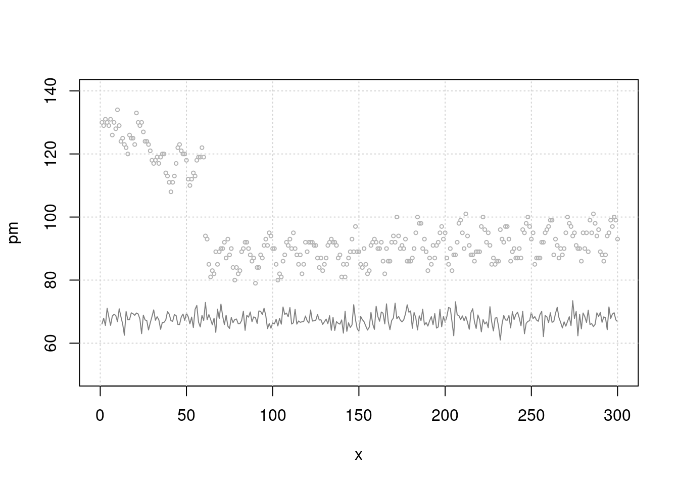
이제 단순 회귀 분석을 해보겠습니다. 어떠한 관계가 관찰되시나요. event 때 많이 사망하고, 미세먼지와는 관련이 없네요. 분명 미세먼지와 관련있게 시뮬레이션 해서 만든 자료인데요. 맞습니다.
lag과seasonality보정이 않되었네요.
## Estimate Std. Error t value Pr(>|t|)
## (Intercept) 90.10455149 6.861474711 13.1319513 2.476263e-31
## x 0.02379324 0.003500538 6.7970236 5.915161e-11
## sin(x/2) -4.41585403 0.308633540 -14.3077581 1.247252e-35
## pm -0.06144597 0.101078610 -0.6079028 5.437196e-01
## event 35.05109683 0.757861036 46.2500315 3.230388e-137그림으로 확인해 보겠습니다. 무언가 잘못 예측이 되고 있죠?
plot(x, pm, type="l", col=grey(0.5), ylim=c(50, 140), xlim=c(0, 300))
grid()
lines(x, death2, col=grey(0.7), type="p", cex=0.5)
mp3 <- c( predict(mt3))
lines(x, mp3, col=75)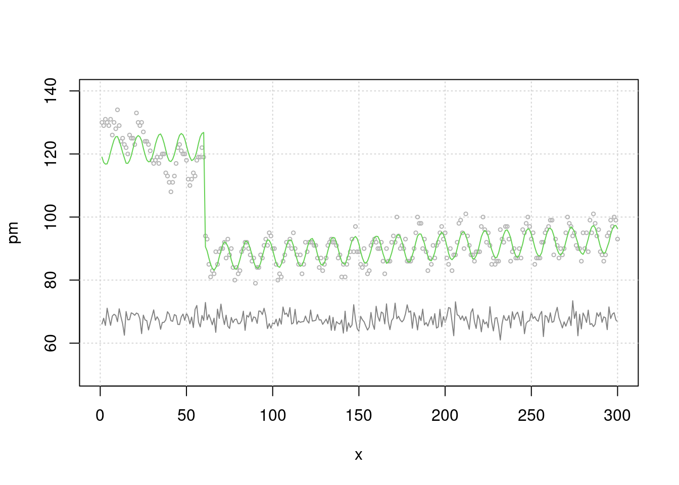
차라리 이렇게 해보는 것은 어떨까요? 시계열적인 요소를 뺀 상태 (residual) 과 미세먼지가 관련이 있나 보는 것입니다 .
mt2 <- glm(death2 ~ x+sin(x/2)+event)
resid_mt2 <-resid(mt2)
risk.m0<-glm(resid_mt2 ~ pm, family=gaussian)
summary(risk.m0)##
## Call:
## glm(formula = resid_mt2 ~ pm, family = gaussian)
##
## Deviance Residuals:
## Min 1Q Median 3Q Max
## -9.6006 -2.2804 -0.1559 2.3275 14.2142
##
## Coefficients:
## Estimate Std. Error t value Pr(>|t|)
## (Intercept) 4.14114 6.79037 0.61 0.542
## pm -0.06128 0.10043 -0.61 0.542
##
## (Dispersion parameter for gaussian family taken to be 14.18007)
##
## Null deviance: 4230.9 on 299 degrees of freedom
## Residual deviance: 4225.7 on 298 degrees of freedom
## AIC: 1650.9
##
## Number of Fisher Scoring iterations: 2risk.mp0 <- c( predict(risk.m0))
plot(pm, resid_mt2, type='p', cex=0.5)
lines(pm, (risk.mp0), col=25)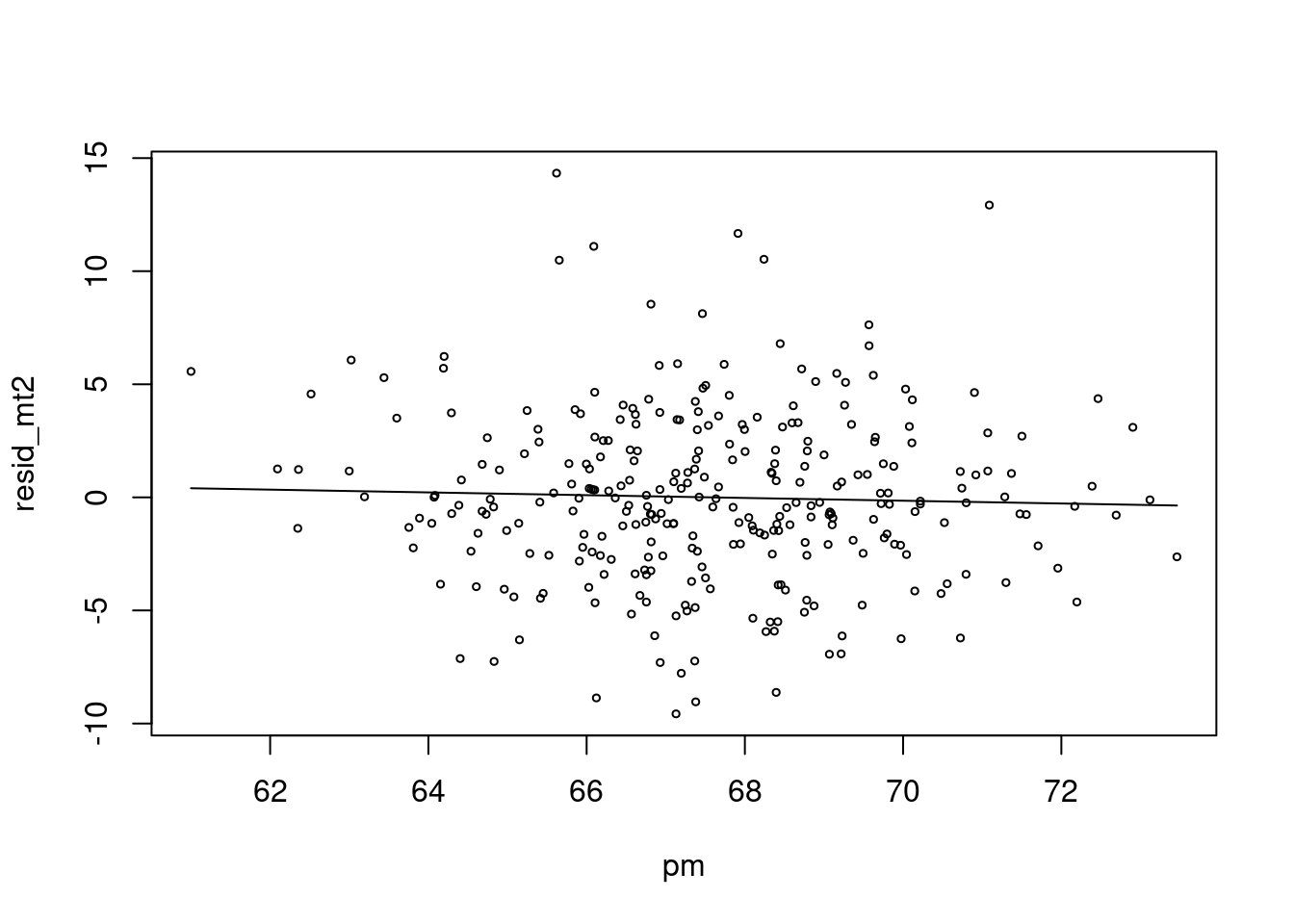
저는 이것이 더 직관적인데요. 심혈관사망에서 시계열적으로 변동이 있는 부분을 뺀 나머지 (residual) 이 pm 이 변동할 때 같이 변동하면 관련성이 있다고 보는 것이지요.
자 이제 lag 을 줘서 관찰해 보겠습니다. lag을 주면 초반 데이터 숫자가 맞지 않는데요. 이때 pm의 평균 값으로 결측치를 대신해서 해결해 보겠습니다.
## [1] 67.57556lag.pm<-6
pm.lag <- c(rep(67.5, lag.pm), pm[1:(length(pm)-lag.pm)])
resid_mt3 <-resid(mt3)
risk.m1<-glm(resid_mt3 ~ pm.lag, family=gaussian)
summary(risk.m1)$coefficients## Estimate Std. Error t value Pr(>|t|)
## (Intercept) -76.437599 5.21757250 -14.65003 5.620794e-37
## pm.lag 1.131554 0.07720006 14.65743 5.276143e-37risk.mp1 <- c( predict(risk.m1))
plot(pm.lag, resid_mt3, type='p', cex=0.5)
lines(pm.lag, risk.mp1, col=25)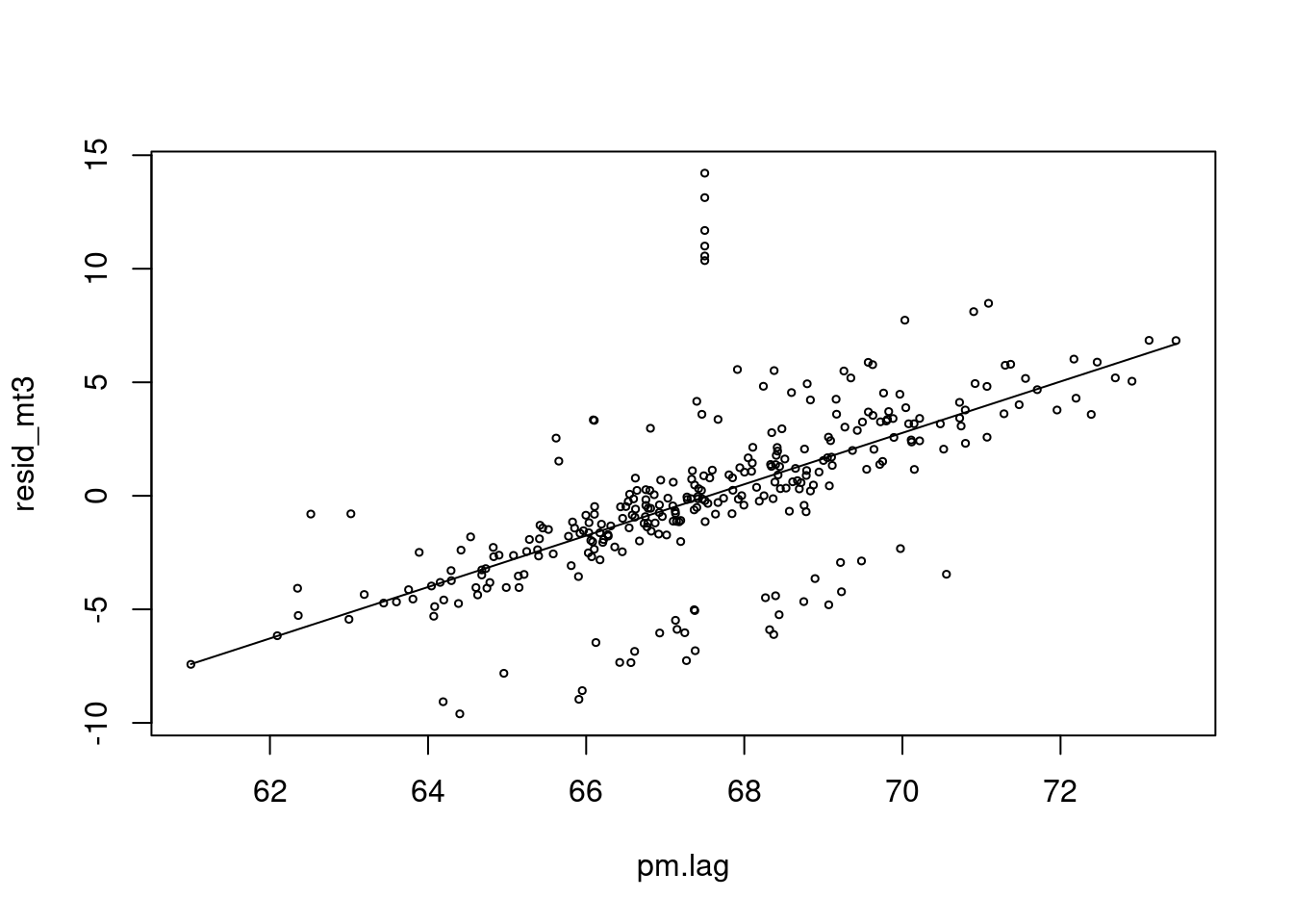
네 이제 pm 과 양의 심혈관 사망에 양의 상관관계가 생겼네요. 우리가 원했던 데이터를 그렇게 만들었었습니다.
> 그림으로 관찰해 보면 빨간색이 lag time을 준것입니다. 누가 더 사망과 관련이 있어 보이나요?
plot(x, resid_mt3, type="l", col=grey(0.5), ylim=c(-15, 40), xlim=c(0, 300))
grid()
lines(x, (pm-50), col=grey(0.7), type="l", cex=0.5)
lines(x, (pm.lag-60), col='red', type="l", cex=0.5)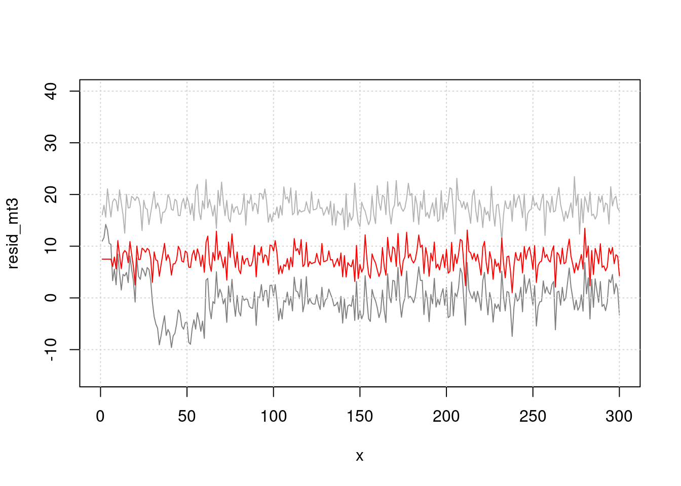
지금 까지 고려한 것은
sin()으로 계절적 요소,lag으로 지연 효과를 고려해서 시계열적 요소를 없앤다음 (residual), pm과 심혈관사망의 관계를 분석하는 방식으로 해보았습니다. 좀더 쉽게 이것을 해보겠습니다.
## Loading required package: nlme##
## Attaching package: 'nlme'## The following object is masked from 'package:dplyr':
##
## collapse## This is mgcv 1.8-33. For overview type 'help("mgcv-package")'.##
## Attaching package: 'mgcv'## The following objects are masked from 'package:gam':
##
## gam, gam.control, gam.fit, smgam<- gam(death2 ~ s(x, bs="cc", k=100)+event, family=gaussian)
p <- predict(mgam)
plot(x, pm, type="l", col=grey(0.5), ylim=c(40, 150), xlim=c(0, 300), cex=2)
grid()
lines(x, death2, col=grey(0.7), type="p", cex=0.5)
legend(x=250, y=70, 'PM10')
legend(x=150, y=65, 'pm10. lag')
legend(x=210, y=110, 'Obs_death')
legend(x=10, y=50, 'Residual(Obs_Death - Gam(fitting)')
lines(x, p)
lines(x, (resid(mgam)+50), col='blue')
lines(x, pm.lag-10, col='red')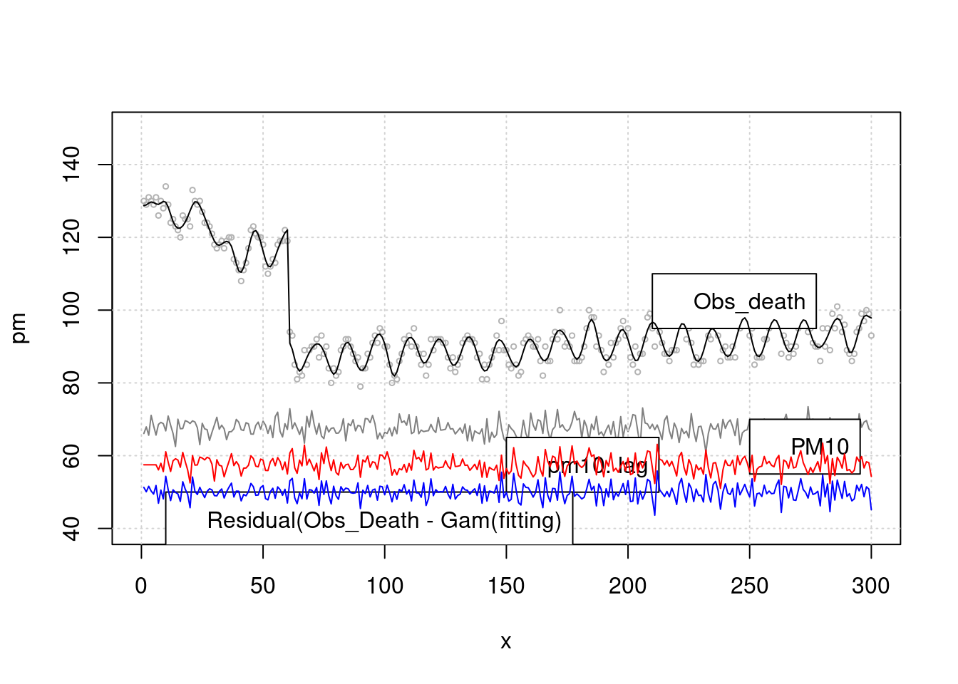 > 이것을 회귀 분석으로 구해보겠습니다. k 가 높을 수록 모형은 어떠한 가요? 네 즉 위에 lag time 과 k 값을 어떻게 조정하는 지를 고려해야 합니다. 우선 lag time 어떻게 찾을 까요?
mgam<- gam(death2 ~ s(x, bs="cc", k=100)+event, family=gaussian)
p <- predict(mgam)
risk.pp1 <-glm(death2 ~ p+pm.lag,family=gaussian)
summary(risk.pp1)$coefficients## Estimate Std. Error t value Pr(>|t|)
## (Intercept) -58.3872771 1.937186312 -30.14025 2.402418e-92
## p 1.0000436 0.004566766 218.98286 0.000000e+00
## pm.lag 0.8642815 0.028266084 30.57663 9.482839e-94## [1] 885.3135mgam150<- gam(death2 ~ s(x, bs="cc", k=10)+event)
p150 <- predict(mgam150)
risk.pp150 <-glm(death2 ~ p150+ pm.lag, family=gaussian)
summary(risk.pp150)$coefficients## Estimate Std. Error t value Pr(>|t|)
## (Intercept) -72.5953393 6.74682944 -10.75992 5.109224e-23
## p150 0.9979243 0.01630871 61.18966 2.087420e-170
## pm.lag 1.0776412 0.09754736 11.04736 5.349868e-24## df AIC
## risk.pp1 4 885.3135
## risk.pp150 4 1629.2747lag 을 찾아 보겠습니다. pm에 대해 lag을 10일까지, 3차 방정식 형태로 구성해 보아라, 그리고 이를 통해 회귀 분석을 시행해 보아라.
library(dlnm)
cb1.pm <-crossbasis(pm, lag=10, argvar=list(fun="lin"),
arglag=list(fun="poly", degree=3))
model1 <-glm(death2 ~ cb1.pm+x+event ,
family=gaussian )
pred1.pm <-crosspred(cb1.pm, model1, at=0:100, bylag=0.1, cumul=TRUE)
plot(pred1.pm, "slices", var=1, col=3, ylab="RR", ci.arg=list(density=15,lwd=2),
#cumul = TRUE,
main="Association with a 1-unit increase in PM10")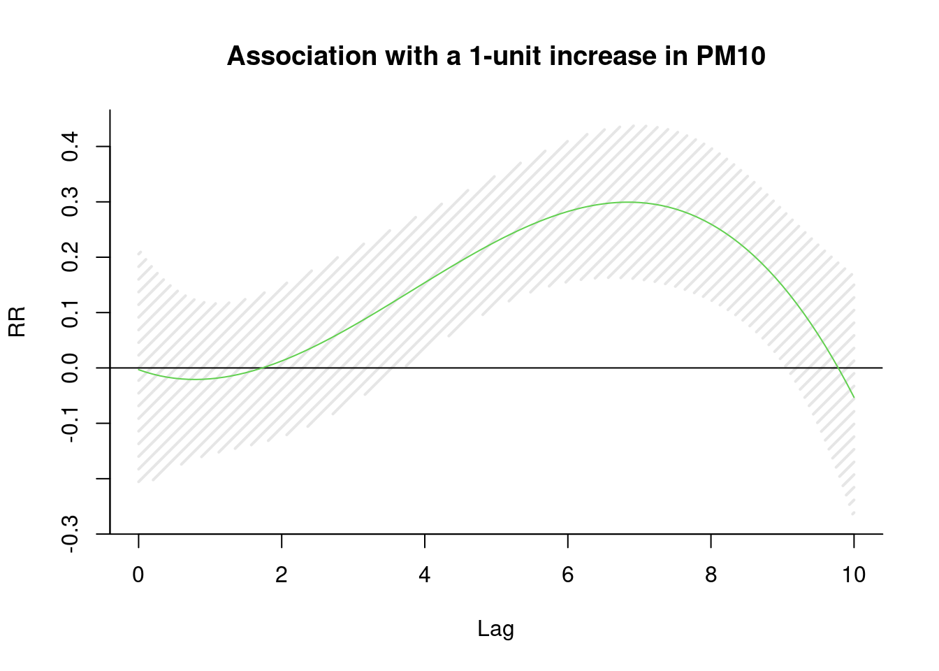
6일을 lag time으로 하면 좋겠네요.
이제 6일을 lag time으로 설정해서 회귀 분석을 수행하면 된다는 것을 알았습니다. 이제 남은 것은 시계열적 요소를 어떻게 찾고, 어떻게 보정할지, 그리고 이 과정을 어떻게 합리적으로 할지 더 논의 하면 됩니다.
13.8 ARIMA
ARIMA (autoregressive intergrated moving average) 는 문자 그대로 자기상관관계와 이동평균을 이용합니다. univariate time series로 보시면 됩니다. ARIMA 모델에서 여러 파라메터를 자동으로 또는 수동으로 설정하여 구성해 가게 됩니다.
ARIMA(p, d, q)를 이해하면서 가 봅겠습니다.
| parameter | content | abbr |
|---|---|---|
| AR | Autoregressive part | p |
| I | Integrateion, degree of differencing | d |
| MA | Moving average part | q |
위 에서 p, d, q를 찾아 가는 방법을 ARIMA 모델이라고 부를 수 있습니다.
lags 과 forecasting errors로 구분할 수 있습니다.
- 과거의 변수가 현재를 예측, autoregressive part
- AR(1) or ARIMA(1,0,0): first order (lag) of AR
- AR(2) or ARIMA(2,0,0): second order (lag) of AR
- 과거의 error 가 현재를 예측 (forecasting error) = moving average part
- MA(1) or ARIMA(0,0,1): first order of MA
- MA(2) or ARIMA(0,0,2): second order of MA
자기상관관계 부분
\[ Y_{t} = c + \Phi_1 Y_{t-1} + \varepsilon_{t} \]
- \(t\) 시간에 관찰되는 변수 (\(Y_{t}\))는
- 상수 (c) 더하기
- 바로 1단위 전 변수 (\(Y_{t-1}\)) 에 계수(coefficient) (\(\Phi\)) 글 곱한 값을 더하고
- 현재의 에러를 \(t (e_{t})\)) 더한다
이동평균 부분
\[ Y_{t} = c + \Theta_1 \varepsilon_{t-1} + \varepsilon_t \]
- \(t\) 시간에 관찰되는 변수 (\(Y_{t}\))는
- 상수 (c) 더하기
- 바로 1단위 전 변수 (\(\varepsilon_{t-1}\)) 에 계수(coefficient) (\(\Phi\)) 글 곱한 값을 더하고
- 현재의 에러를 \(t (e_{t})\)) 더한다
결국 자기 상과관계와 이동평균을 한꺼번에 사용하면 아래와 같습니다.
\[\begin{align*} y_t &= \phi_1y_{t-1} + \varepsilon_t\\ &= \phi_1(\phi_1y_{t-2} + \varepsilon_{t-1}) + \varepsilon_t\\ &= \phi_1^2y_{t-2} + \phi_1 \varepsilon_{t-1} + \varepsilon_t\\ &= \phi_1^3y_{t-3} + \phi_1^2 \varepsilon_{t-2} + \phi_1 \varepsilon_{t-1} + \varepsilon_t\\ \end{align*}\]
d 는 시계열그림에서 ACF, PACF의 형태를 보고 차분의 필요여부 및 차수를 d를 결정하고 AR차수와 MA차수를 결정
어떻게 p, d, q 를 구할수 있을 까요, 다음 장을 보겠습니다.