Chapter 9 graphs for public health II
9.1 Data Visualization example (EEG data)
In public health, another most common used data is bio-signal data. Bio-signal data usually used in medical research, but recently bio-log signals are widely used in public health beyond medical setting. Now I present some example of data visualization using bio-signal data from EEG.
9.2 Introduction
EEG refers to the signal of the brain’s electrical activty. Electrodes are placed on the scalp, and each electrodes recorded brain’s activity. EEG is one of the most common methods to support diagnosis of brain diseases such as epilepsy, sleep disorder and even brain death. Furthermore, we can get usufull understand how brain activity correlated to various neurological activity. So, I tried to anaysis EEG signal and hope to predict eye opening status.
The data include information of row_n, AF3, F7, F3, FC5, T7,P7, O1, O2, P8, T8, FC6, F4, F8, AF4, and eyeDetection. Eye Detection is outcome variable data Open or Closed. Others numeric variable about activity of each electrodes. Each electro-nodes place on scalp, and represent area of particular location on brain, as below.
rm(list=ls())
url <- "https://upload.wikimedia.org/wikipedia/commons/thumb/7/70/21_electrodes_of_International_10-20_system_for_EEG.svg/1024px-21_electrodes_of_International_10-20_system_for_EEG.svg.png"
download.file(url, 'images/eegpng.png')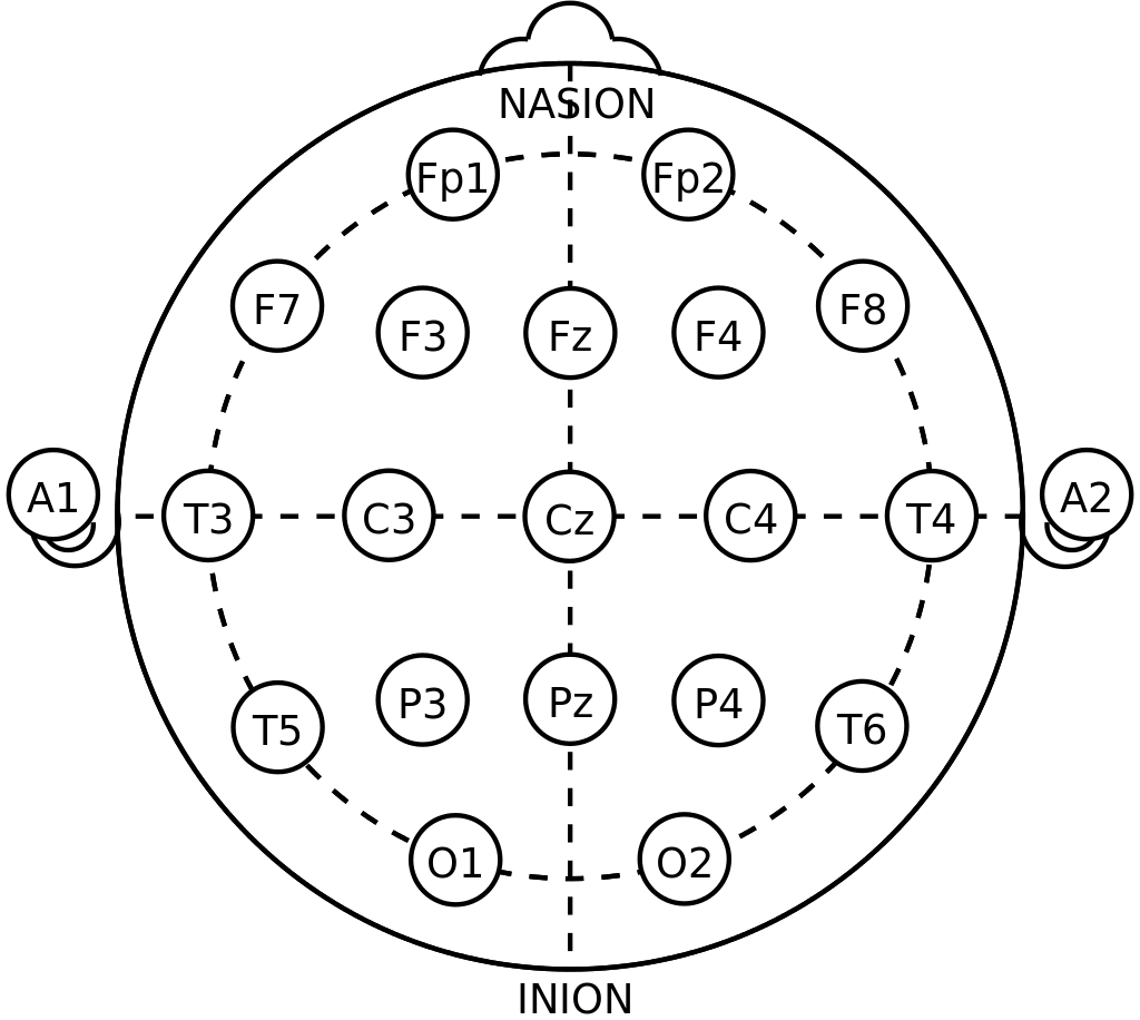
eeg electrodes from wiki
9.3 Dataset and Data step
9.3.1 video
| my video url is |
|---|
| https://youtu.be/JJl5l5yRKj8 |
9.3.2 Data download and handling
The data set locate here, https://archive.ics.uci.edu/ml/machine-learning-databases/00264/EEG%20Eye%20State.arff.
The data was stored into my computer, as name of ‘dl_eeg.txt’ in `data’ folder.
url ='https://archive.ics.uci.edu/ml/machine-learning-databases/00264/EEG%20Eye%20State.arff'
download.file(url, 'data/dl_eeg.txt')
To start the data step, some packages should be loaded.
library(tidyverse)
#library(caret)
library(knitr)
library(kableExtra)
library(htmlTable)
#library(doMC)
scan the data and creat DB for analysis
## [1] 48dat<-mm[-c(1:48)]
book <- mm[1:48]
book[-c(1:2, 48)] %>%
matrix(., ncol=3, byrow=TRUE) %>%
.[,2] -> col_names
col_names## [1] "AF3" "F7" "F3" "FC5" "T7"
## [6] "P7" "O1" "O2" "P8" "T8"
## [11] "FC6" "F4" "F8" "AF4" "eyeDetection"the tibble form is easy to hand or transforming. So, I change the data form to tibble style.
tibble(wave =dat) %>%
  mutate (val = strsplit(wave, ","), row_n=row_number()) %>%
  unnest (cols=c(val)) %>%
  select (-wave) %>%
  mutate (val = as.numeric(val)) %>%
  group_by(row_n)  %>%
  mutate (wave_colname = col_names) %>%
  ungroup() %>%
  spread (key = wave_colname, value = val, fill = 0,convert = FALSE) %>%
  select (row_n, col_names) %>%
  arrange (row_n) ->
  eeg
I check the class of all variable.
##  [1] "row_n"        "AF3"          "F7"           "F3"           "FC5"
##  [6] "T7"           "P7"           "O1"           "O2"           "P8"
## [11] "T8"           "FC6"          "F4"           "F8"           "AF4"
## [16] "eyeDetection"## row_n AF3 F7 F3 FC5 T7
## "numeric" "numeric" "numeric" "numeric" "numeric" "numeric"
## P7 O1 O2 P8 T8 FC6
## "numeric" "numeric" "numeric" "numeric" "numeric" "numeric"
## F4 F8 AF4 eyeDetection
## "numeric" "numeric" "numeric" "numeric"This data were measure for 117 seconds, I create sec variable to represent measurement time. I create facotor variable for eye opening status `Eye’, as below.
eeg <- eeg %>%
  mutate(Eye = ifelse(eyeDetection ==1, 'open', 'closed')) %>%
  mutate(sec = seq(0, 117, length.out = nrow(.)))
For data step, the long form data were created via gather function. the key represent each electrode, and the activity were stored into activity variable. EyeDetection, row_n, sec, Eye will be indentical variable for each electrode activity.
eeg %>%
  gather(key = 'electrode', value = 'activity', -eyeDetection, -row_n, -sec, -Eye) ->
  eegl
eegl %>% head()
## # A tibble: 6 x 6
## row_n eyeDetection Eye sec electrode activity
## <int> <dbl> <chr> <dbl> <chr> <dbl>
## 1 1 0 closed 0 AF3 4329.
## 2 2 0 closed 0.00781 AF3 4325.
## 3 3 0 closed 0.0156 AF3 4328.
## 4 4 0 closed 0.0234 AF3 4329.
## 5 5 0 closed 0.0312 AF3 4326.
## 6 6 0 closed 0.0391 AF3 4321.9.3.3 data explorer
9.3.3.1 heatmap
9.3.3.1.1 video 2
| my video url is |
|---|
| https://youtu.be/X-ybmSlDPfI |
The heatmap can show overview the time course about eye opening status. Dark blue indicate closed status, and light blue indicate eye open status.
eegl %>%
ggplot(aes(x = sec, y = 0.5, fill = eyeDetection)) +
geom_tile() +
scale_fill_continuous(name = "Eye status",
limits = c(0, 1),
labels = c('closed',"transit", 'open'),
breaks = c(0,0.5, 1)) +
theme_classic() +
scale_y_continuous(breaks = c(0, 0.5, 1), 'Eye status') +
scale_x_continuous(breaks = c(0, 30, 60, 90, 117)) +
theme(aspect.ratio=1/7)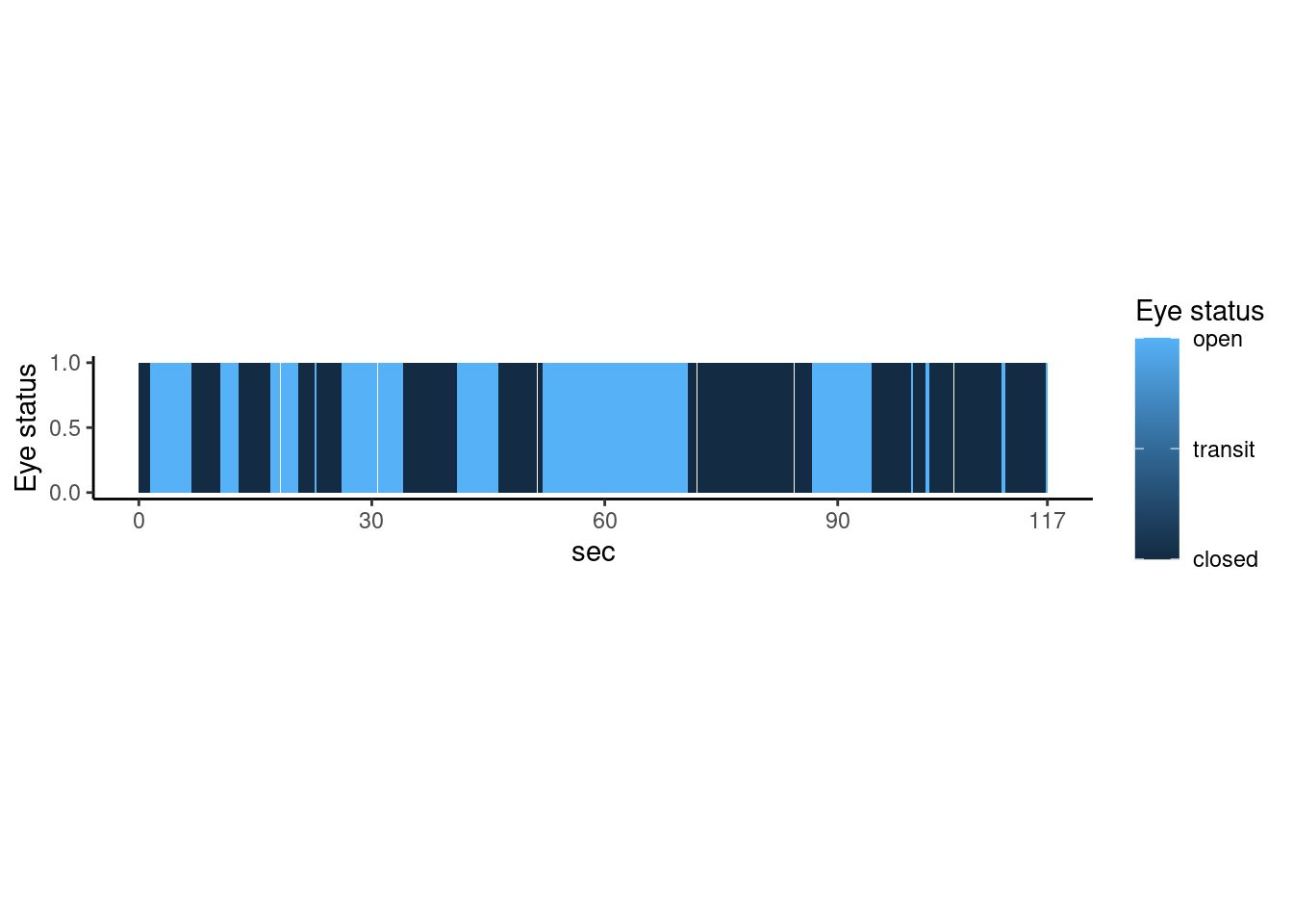 #### waveform
9.3.3.1.2 video 3
| my video url is |
|---|
| https://youtu.be/75aaK-qRP2s |
The activity waves are plotting for data explorer.
eegl %>%
ggplot(aes(x = row_n, y = activity, color = Eye)) +
geom_line(size = c(1)) +
geom_point(alpha = 1)+
facet_grid(electrode ~. ) +
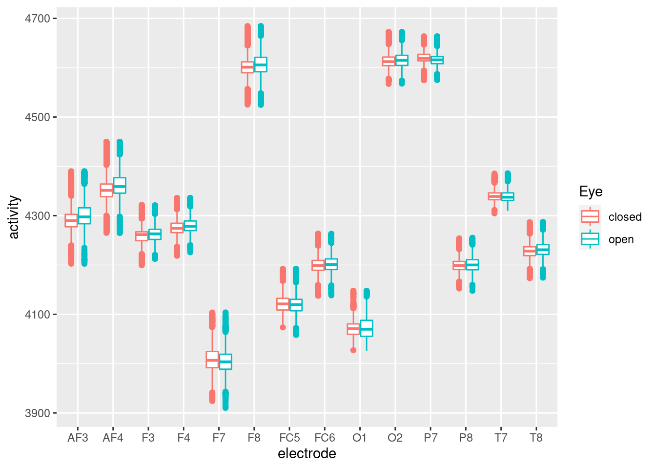
theme_classic() 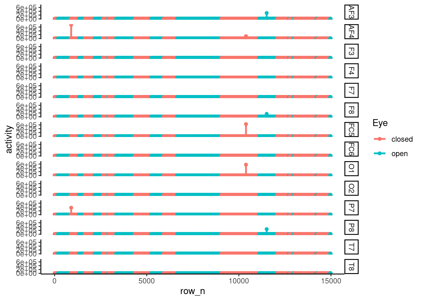 There are much of outlier, so the fluctuation of each node’s activity atteunted. So We needed to exclude outlier. To ensure the outlier status, I plot the boxplot, as below. The boxplot also suggested that there were much of outlier effect.
eegl %>%
ggplot(aes(x = electrode, y = activity, color = Eye)) +
geom_boxplot() +
scale_y_continuous(trans='log2') +
theme_classic()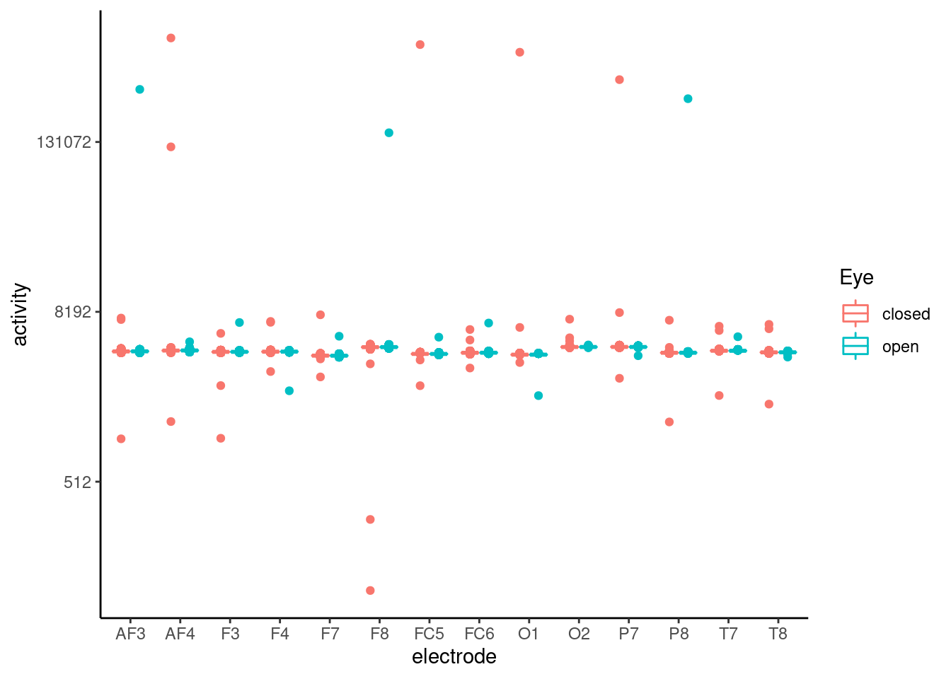 Althoug there are outlier effect on data, but I just want to check the
 t-test results.
ttest<- eegl %>% select(-eyeDetection, -row_n) %>%
  group_by(electrode)  %>%
  nest() %>%
  mutate(stats     = map(data, ~t.test(activity ~ Eye, data=.x)),
         summarise = map(stats, broom::glance))  %>%
  select(electrode, summarise) %>%
  unnest(summarise)
ttest %>%
  mutate_if(is.numeric, round, 2) %>%
  mutate(p.values = ifelse(p.value <0.01, '<0.01', as.character(p.value))) %>%
  select(electrode,`difference` = estimate, 'open' = estimate1, 'closed' =  estimate2, p.values) %>%
  htmlTable(
    cgroup=c("", "Eye status", ""),
    n.cgroup=c(2, 2, 1),
    caption = "Table1. t-test result without outlier cleaning",
    align = 'llrc'
  )
## `mutate_if()` ignored the following grouping variables:
## Column `electrode`| Table1. t-test result without outlier cleaning | |||||||
| Eye status | |||||||
|---|---|---|---|---|---|---|---|
| electrode | difference | open | closed | p.values | |||
| 1 | AF3 | -52.4 | 4298.4 | 4350.8 | 0.25 | ||
| 2 | F7 | 7.39 | 4013.08 | 4005.69 | <0.01 | ||
| 3 | F3 | -3.47 | 4262.46 | 4265.94 | <0.01 | ||
| 4 | FC5 | 78.98 | 4200.39 | 4121.41 | 0.31 | ||
| 5 | T7 | 0.03 | 4341.75 | 4341.73 | 0.96 | ||
| 6 | P7 | 46.13 | 4664.73 | 4618.59 | 0.29 | ||
| 7 | O1 | 66.82 | 4140.39 | 4073.57 | 0.33 | ||
| 8 | O2 | -1.48 | 4615.39 | 4616.87 | <0.01 | ||
| 9 | P8 | -41.13 | 4200.37 | 4241.5 | 0.29 | ||
| 10 | T8 | -3.61 | 4229.7 | 4233.31 | <0.01 | ||
| 11 | FC6 | -4.88 | 4200.26 | 4205.15 | <0.01 | ||
| 12 | F4 | -4.01 | 4277.43 | 4281.44 | <0.01 | ||
| 13 | F8 | -31.88 | 4600.9 | 4632.77 | 0.15 | ||
| 14 | AF4 | 89.42 | 4456.57 | 4367.15 | 0.31 | ||
9.3.4 data cleaning for outlier
The interquartile range is useful for detecting the presence of outliers. Outliers are individual values that fall outside of the overall pattern of a data set. So, the outlier can be define when they are far way as several times of interquarile range from median. I made scale_median function to detect outlier. ther are several step to make function. first, calculate the interquartile range. The differece between median and value divided by inter quartile range, and the absolute value will be Z-score. That z-score mean how many times of interquartile range far from median. I used 2.5 times for detect outlier.
scale_median <- function(x){
    Q1  <- quantile(x, 0.25)
    Q3  <- quantile(x, 0.75)
    iqr <- c(Q3 - Q1)
  ifelse(x < median(x),(x - Q1)/iqr*-1,(x - Q3)/iqr*1 )
}
eegl1<-
  eegl %>%
  group_by(electrode) %>%
  nest() %>%
  mutate(Zscores = map (data, ~scale_median(.$activity))) %>%
  unnest(cols = c(data, Zscores))  %>%
  filter(Zscores < 2.5) #Outlier is Zscores > 2.5 or <-2.5
I check box-plot without outlier. That plot sounds good for me. So, I can generate wave form plot.
 Here, I plot wave form of each electrodes’ activity. Before generate the wave plot, I want increase the working cores.
## [1] 1My computer use only 1 core, so I increse nubmer of cores working upto 11 cores.
## [1] 31Then, I want plot wave form.
eegl1 %>%
  ggplot(aes(x = sec, y = activity, fill = eyeDetection)) +
  geom_point(size = 0.1, alpha =0.5) +
  geom_line(aes(color = eyeDetection), show.legend = F) +
  facet_grid(electrode ~., scales = "free" ) +
  theme_classic() +
  scale_fill_continuous(name = "Eye status", limits = c(0, 1),
                        labels = c('close', 'open'), breaks = c(0, 1)) +
  xlab('Time series') +
  scale_x_continuous(breaks = c(0, 30, 60, 90, 117))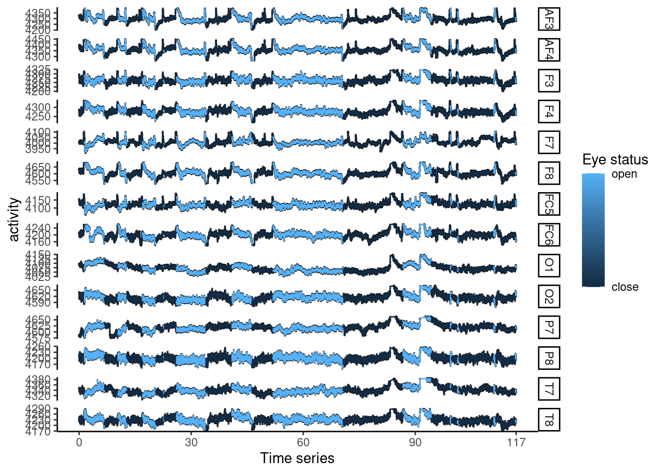
9.3.5 Data reshape (longform and wideform)
Now, I can confirm the cleaer data set without outlier. I attached 0 behind to data name to figure out the clear data. I also creat wide form data, too.
eegw0 <- eegl1 %>% select(-Zscores) %>%
  spread(key = electrode, value = activity) %>%
  drop_na()

eegl0 <- eegw0 %>% select(-row_n) %>%
  gather(key = electrode, value = activity, -c(eyeDetection,Eye, sec) )
names(eegl0)
## [1] "eyeDetection" "Eye" "sec" "electrode" "activity"9.4 Data analysis
9.4.1 video
| my video url is |
|---|
| https://youtu.be/EGPoJ7nHrpU |
9.4.2 data splite
I splite traing and testing date set using 80% of eye open for training set.
library(caret)
set.seed(1)
dfs <-eegw0 %>%select(-eyeDetection, -sec, -row_n)

trainIndex <- createDataPartition(dfs$Eye, p = 0.8,
                                  list = FALSE,
                                  times= 1) %>% as.vector()

training <- dfs[ trainIndex, ]
testing  <- dfs[-trainIndex, ]
There are 5924 points for eye closed, and 4912 points for eye open.
| Eye | n | |
|---|---|---|
| 1 | closed | 5924 |
| 2 | open | 4912 |
9.4.3 First gbm algorithm
I choose Gradient boosting machine learning (gbm) technique for classification problem. I search various algorithm in basic tunning by caret package. Among them(parRF, naive_bayes, knn, lssvmPoly, svmLinearWeights, gbm, brnn, regLogistic, OneR, RFlda, qda, glm, LogitBoost), the gbm technique show greatest performance.
The gbm is one of the decision trees methods with boosting methods. For detain, I get information from http://uc-r.github.io/gbm_regression. Now, I start my first gbm model
gbmFit1 <-train(Eye ~., data = training,
                method = 'gbm',
                #preProc = c("center", "scale")
                )
dt <-Sys.time()
gbmFit1$results %>%tibble()%>%
  pull(Accuracy) %>%max() %>%round(., 3)->
  model_accuracy

a1<-confusionMatrix(predict(gbmFit1, newdata = testing), as.factor(testing$Eye))
results_table <- tibble(
  Methods = "first gbm method",
  Accuracy = model_accuracy,
  Accuracy_in_test = round(a1$overall[[1]], 3))
My first gbm method show 0.798 of accuracy in training, it is not bed. The confusion matrix report results in testing set. The Accuracy is 80%, Sensitivity is 84.9%, and Specificity is 74%.
| Methods | Accuracy | Accuracy_in_test | |
|---|---|---|---|
| 1 | first gbm method | 0.798 | 0.792 |
TestResult <- predict(gbmFit1, newdata = testing)
confusionMatrix(TestResult, as.factor(testing$Eye))
## Confusion Matrix and Statistics
##
## Reference
## Prediction closed open
## closed 1258 341
## open 223 886
##
## Accuracy : 0.7917
## 95% CI : (0.7759, 0.8069)
## No Information Rate : 0.5469
## P-Value [Acc > NIR] : < 2.2e-16
##
## Kappa : 0.5763
##
## Mcnemar's Test P-Value : 8.368e-07
##
## Sensitivity : 0.8494
## Specificity : 0.7221
## Pos Pred Value : 0.7867
## Neg Pred Value : 0.7989
## Prevalence : 0.5469
## Detection Rate : 0.4645
## Detection Prevalence : 0.5905
## Balanced Accuracy : 0.7858
##
## 'Positive' Class : closed
## gbmFit3 creates a new summary data set with var, factors in our model, and its relative influence (rel.inf) each variable had on eye opening status. O1 and P7, F8, F7 show highest rel.infs.
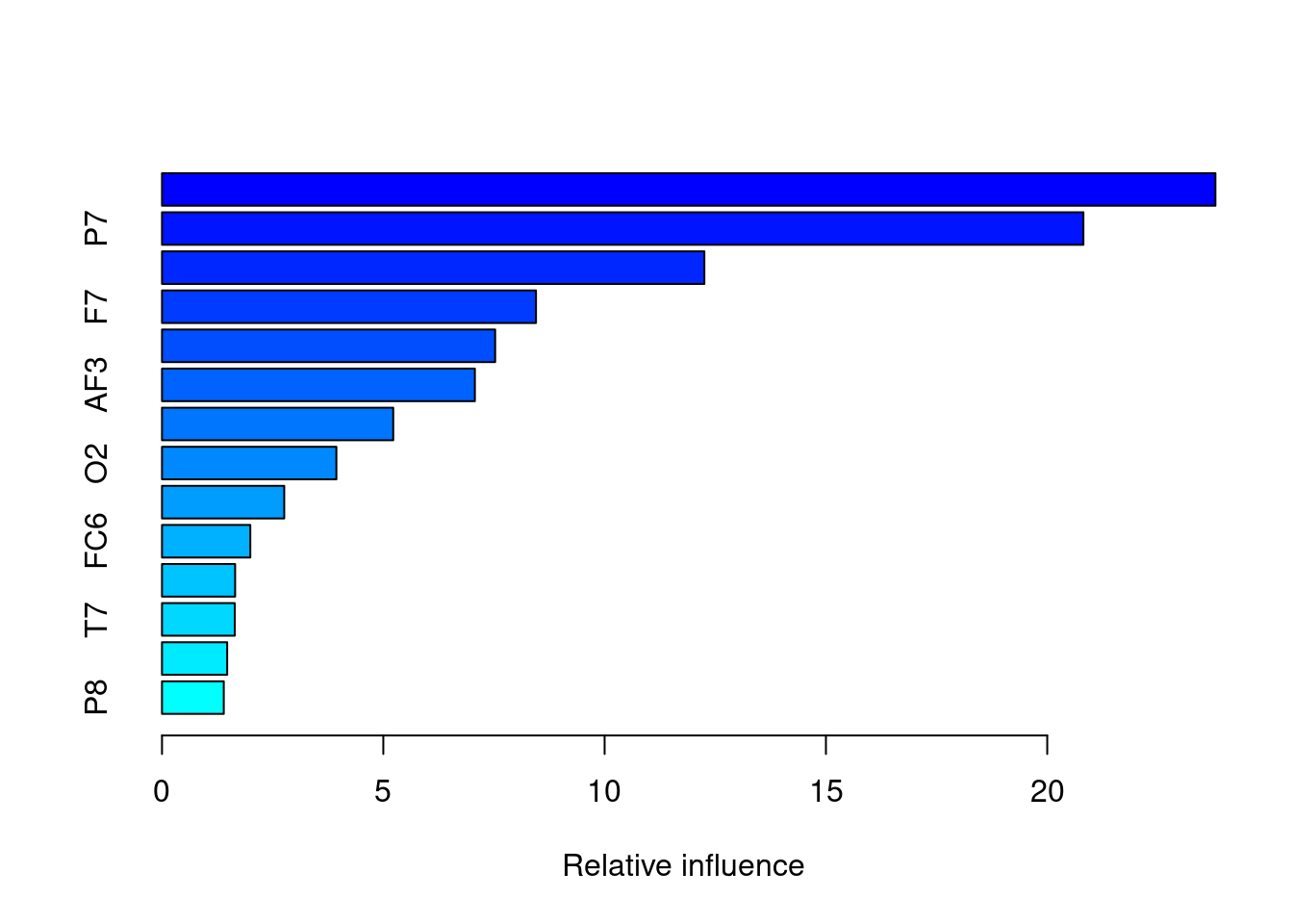
##     var   rel.inf
## O1   O1 23.799686
## P7   P7 20.817368
## F8   F8 12.253765
## F7   F7  8.449242
## AF4 AF4  7.527027
## AF3 AF3  7.068717
## F4   F4  5.224236
## O2   O2  3.939794
## T8   T8  2.761357
## FC6 FC6  1.995400
## FC5 FC5  1.652006
## T7   T7  1.643377
## F3   F3  1.472344
## P8   P8  1.395682
I search classification algorithms, and find parRF, naive_bayes, knn, lssvmPoly, svmLinearWeights, gbm, brnn, regLogistic, OneR, RFlda, qda, glm, LogitBoost algorithm. Among them, “parRF”, “naive_bayes”, “knn”,“svmLinearWeights”, “gbm”,“regLogistic”,“glm”,“LogitBoost” are chosen for data analysis due to some error for package install and load library in caret package. Among them, knn and gbm show higest accuracy I just compare the knn in current report.
set.seed(1)
dfs <-eegw0 %>%select(-eyeDetection, -sec, -row_n)

trainIndex <- createDataPartition(dfs$Eye, p = 0.8,
                                  list = FALSE,
                                  times= 1) %>% as.vector()

training <- dfs[ trainIndex, ]
testing  <- dfs[-trainIndex, ]

fitControl <- trainControl(
  # 10 -fold Cross Validation
  method = "repeatedcv",
  number = 10,
  # repeated 10 times
  repeats = 10
)
st <-Sys.time()
knnFit1 <- train (Eye ~ ., data=training,
                  method    = 'knn',
                  #preProc = c("center", "scale"),
                  trControl = fitControl)
et <-Sys.time()
et-stknnFit1$results %>%tibble()%>%
pull(Accuracy) %>%max() %>%round(., 3)->
model_accuracy
a6<-confusionMatrix(predict(knnFit1, newdata = testing), as.factor(testing$Eye))
a6## Confusion Matrix and Statistics
##
## Reference
## Prediction closed open
## closed 1441 53
## open 40 1174
##
## Accuracy : 0.9657
## 95% CI : (0.9581, 0.9722)
## No Information Rate : 0.5469
## P-Value [Acc > NIR] : <2e-16
##
## Kappa : 0.9306
##
## Mcnemar's Test P-Value : 0.2134
##
## Sensitivity : 0.9730
## Specificity : 0.9568
## Pos Pred Value : 0.9645
## Neg Pred Value : 0.9671
## Prevalence : 0.5469
## Detection Rate : 0.5321
## Detection Prevalence : 0.5517
## Balanced Accuracy : 0.9649
##
## 'Positive' Class : closed
## The accuracy of knn is 0.9656573 in testing set, it is almost same to gbm method.
I trie to predict eye opening status using electronode, although I created some new variable from original data but they did not increse the model performance. The time seriese slice did not improve the model performance, either. The electrodne activity can predict eye opening statys about accuracy 94% in gbm and knn model. However I hope to test other algorithms such as parRF, naive_bayes, knn, lssvmPoly, svmLinearWeights, gbm, brnn, regLogistic, OneR, RFlda, qda, glm, LogitBoost in near future.