Chapter 6 Plots and Tables for public health

6.1 데이터표 준비

데이터 변형을 실습 자료인 2017년 근로환경조사 자료를 통해 실습할 것입니다.. 자료는 안전보건공단, 근로환경조사 원시자료 사이트 (http://kosha.or.kr/kosha/data/primitiveData.do) 에서 신청할 수 있습니다.. 시각화는 표와 그래프 둘을 다룰 것이고, 표는 보건학에서 주로 사용하는 표1,2,3과 그래프는 막대 그래프부터 시계열 자료까지 나타내도록 하겠습니다. 실습에 필요한 라이브러리를 불러오겠습니다.

library(devtools)
library(Table1) 
library(ggplot2)
library(tidyverse)
library(htmlTable)
library(haven)
library(gmodels)

6.2 ggplot basic

기본적인 표와 그래프를 그리기 앞서, 가장 많이 사용되는 package인 ggplot2 에 대해 알아 보겠습니다. 내장된 데이터인 iris데이터를 이용해 실습하겠습니다.

data(iris)

6.2.1 그래프 틀

그래프를 그리기 위해서 필요한 것은 데이터, x-axis, y-axis 입니다. 이를 통해 틀을 만들고 이후 필요한 것들을 추가하는 방식입니다.

iris %>% # 데이터 선정
  ggplot(aes(x = Sepal.Length, y = Sepal.Width))

# aes 안에 x축, y축 설정

이렇게 X, Y -axis 가 만들어 졌습니다. xlab, ylab을 통해 축 이름과 ggtitle을 통해 제목을 바꾸어 보겠습니다.

iris %>% # 데이터 선정
  ggplot(aes(x = Sepal.Length, y = Sepal.Width)) +
# aes 안에 x축, y축 설정
  xlab("잎 길이 (sepal length") + ylab("잎 넓이 (sepal width") +
  ggtitle("잎의 길이 넓이에 따른 아이리스 꽃 분류")

6.2.2 레이어

레이어는 틀 안에 무엇을 넣을 지 입니다. geom_x() 형식 입니다. x에는 point, line, smooth, histogram, density, boxplot, bar 가 있습니다.

geom_x()	내용
geom_point()	scatter plot, 산점도
geom_line()	line plot, 선
geom_smooth()	prediction line, 예측선
geom_histogram()	histogram, 히스토그래프
geom_density()	density line, 밀도함수
geom_boxplot()	boxplot plot, 박스표
geom_bar()	bar chart, 막대그래프

6.2.2.1 geom_point()

iris %>% # 데이터 선정
  ### 기본 설정 
  ggplot(aes(x = Sepal.Length, y = Sepal.Width)) +
  xlab("잎 길이 (sepal length") + 
  ylab("잎 넓이 (sepal width") +
  ggtitle("잎의 길이 넓이에 따른 아이리스 꽃 분류") +
  ### 레이어
  geom_point()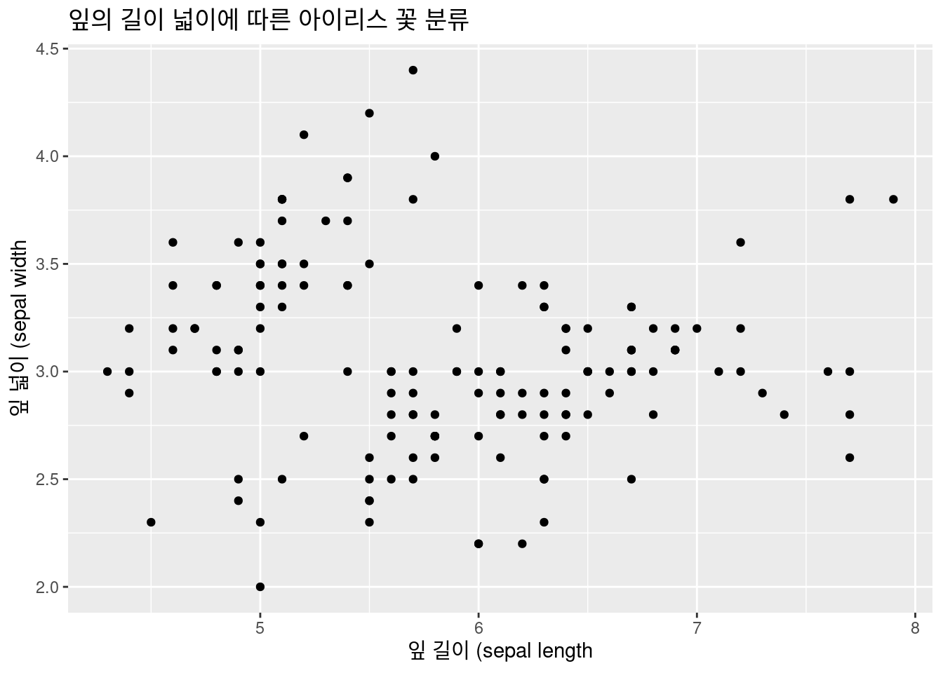

좀더 나아가 보겠습니다. 산점도로 구별이 되지 않습니다. 이때 아이리스 종류 별로 색을 다르게 해보겠습니다. aes( ) 안에 color = Species 를 넣어 틀을 만들겠습니다.

iris %>% # 데이터 선정
  ### 기본 설정 
  ggplot(aes(x = Sepal.Length, y = Sepal.Width, 
             color = Species)) + # 색 구별 추가!
  xlab("잎 길이 (sepal length") + 
  ylab("잎 넓이 (sepal width") +
  ggtitle("잎의 길이 넓이에 따른 아이리스 꽃 분류") +
  ### 레이어
  geom_point()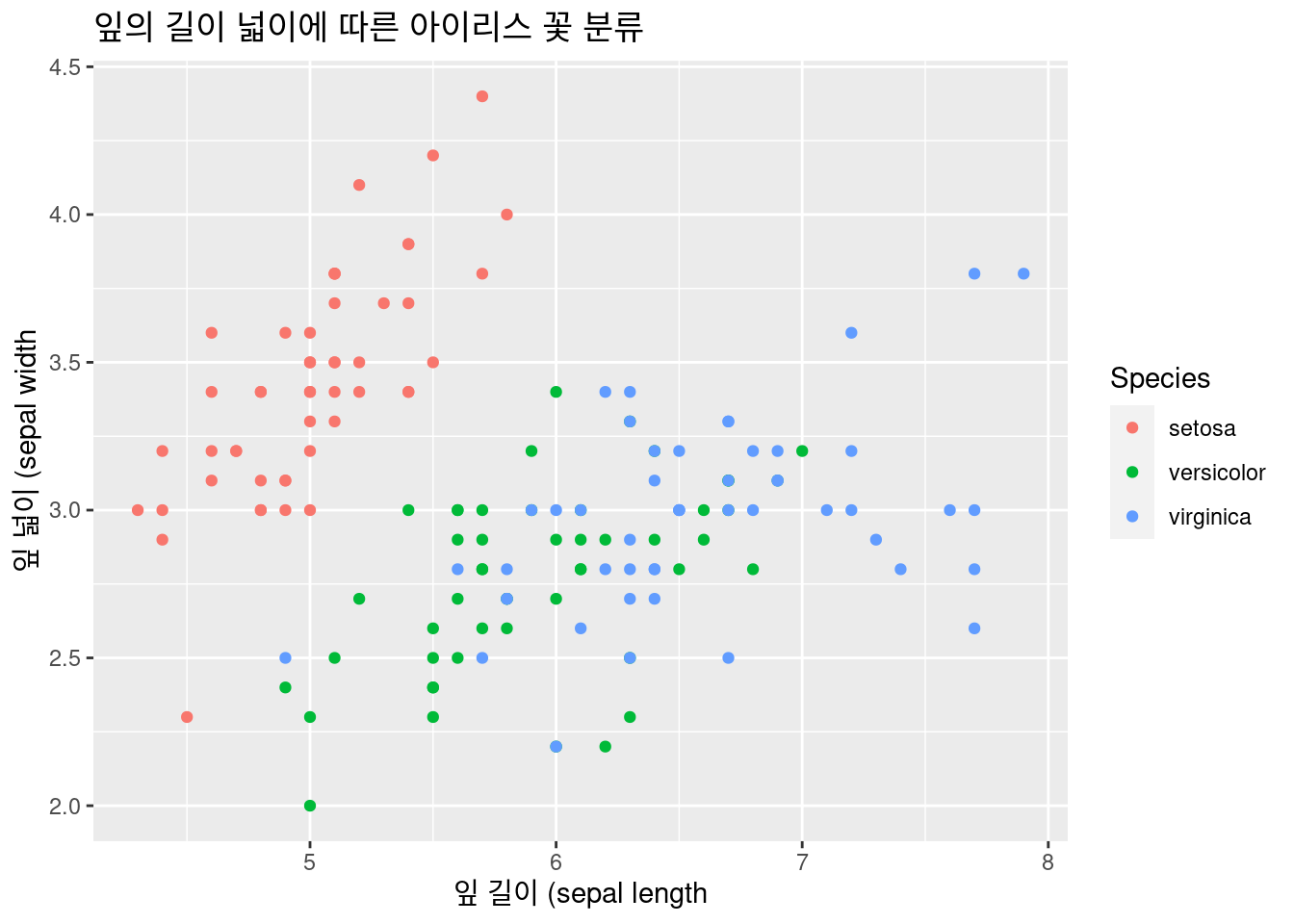

어떻나요? 조금더 좋아졌습니다. 이번에는 추세선 geom_smooth() 를 추가하여 종류별로 잎의 길이와 넓이와의관계를 보겠습니다. geom_line() 도 추가해 보세요. 여기서는 논리적으로 효용성이 없어 생략하겠습니다 .

6.2.2.2 geom_smooth()

iris %>% # 데이터 선정
  ### 기본 설정 
  ggplot(aes(x = Sepal.Length, y = Sepal.Width, 
             color = Species)) + # 색 구별 추가!
  xlab("잎 길이 (sepal length") + 
  ylab("잎 넓이 (sepal width") +
  ggtitle("잎의 길이 넓이에 따른 아이리스 꽃 분류") +
  ### 레이어
  geom_point() + # geom_line() +
  geom_smooth() # 추세선 추가

## `geom_smooth()` using method = 'loess' and formula 'y ~ x'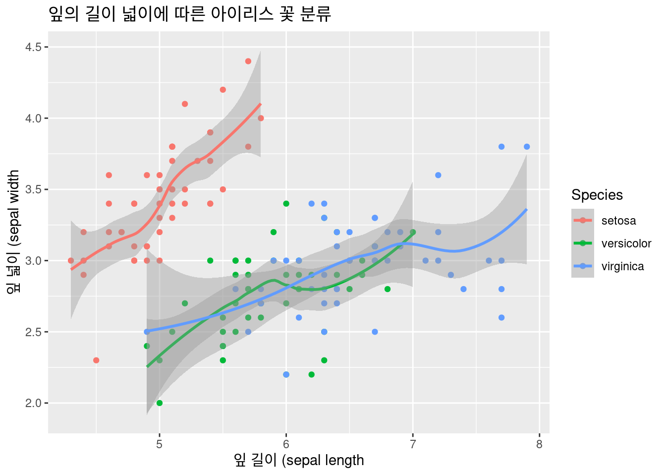

선형 추세성을 추가하고, 5차방정식 추세선도 추가해 보겠습니다 .

iris %>% # 데이터 선정
  ### 기본 설정 
  ggplot(aes(x = Sepal.Length, y = Sepal.Width, 
             color = Species)) + # 색 구별 추가!
  xlab("잎 길이 (sepal length") + 
  ylab("잎 넓이 (sepal width") +
  ggtitle("잎의 길이 넓이에 따른 아이리스 꽃 분류") +
  ### 레이어
  geom_point() +
  geom_smooth(method = 'lm', formula = y ~ poly(x, 5), se = FALSE, linetype = 1) +
  geom_smooth(method = 'lm', formula = y ~ x, se = FALSE, linetype = 2)  # 추세선 추가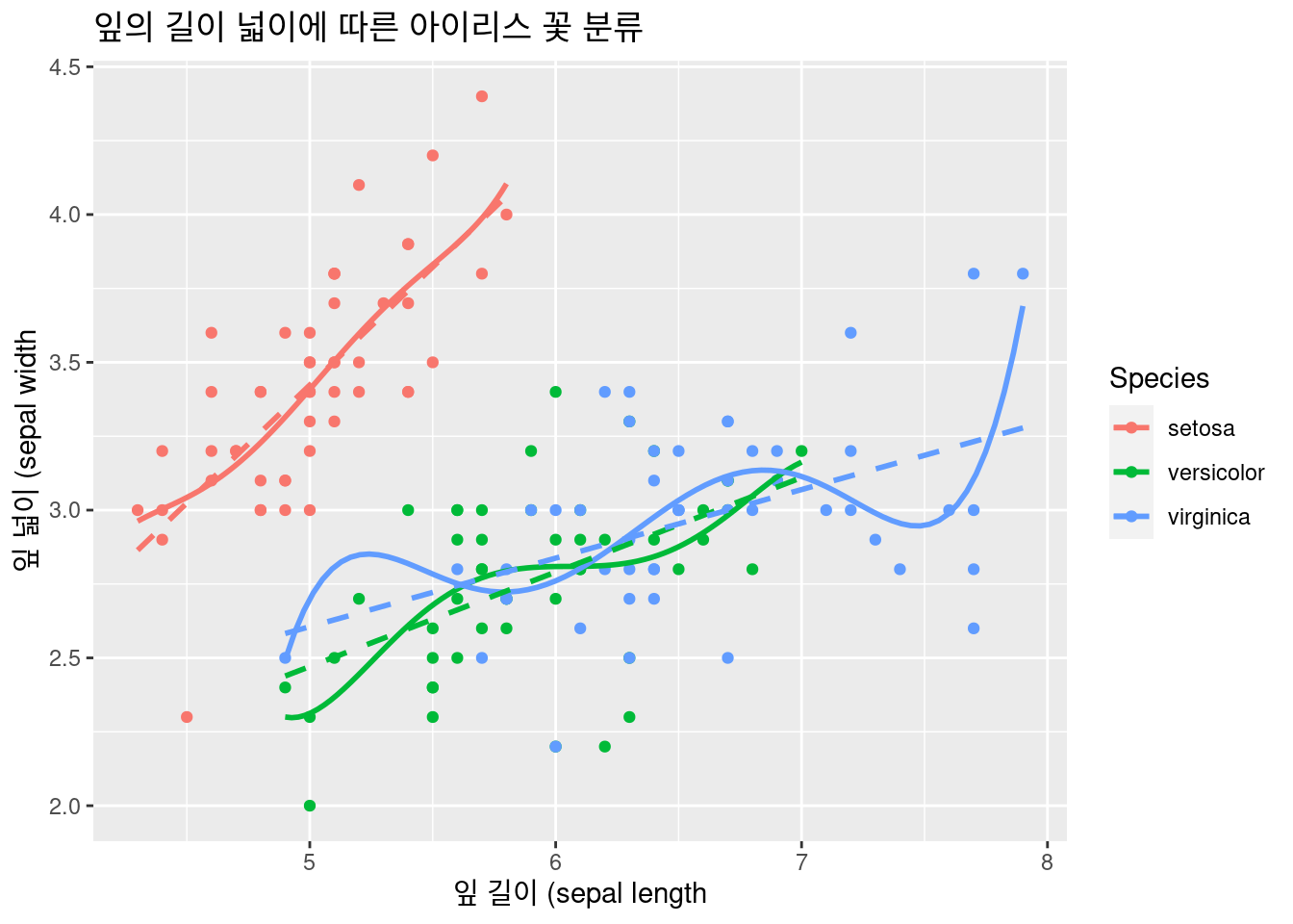

##### faceting

한 화면에 그렸더니 장점도 있지만, 복잡한 부분도 있습니다. 이럴 때는 faceting 을 이용합니다. facet_wrap()

iris %>% # 데이터 선정
  ### 기본 설정 
  ggplot(aes(x = Sepal.Length, y = Sepal.Width, 
             color = Species)) + # 색 구별 추가!
  xlab("잎 길이 (sepal length") + 
  ylab("잎 넓이 (sepal width") +
  ggtitle("잎의 길이 넓이에 따른 아이리스 꽃 분류") +
  ### 레이어
  geom_point() +
  geom_smooth(method = 'lm', formula = y ~ poly(x, 5), se = FALSE, linetype = 1) +
  geom_smooth(method = 'lm', formula = y ~ x, se = FALSE, linetype = 2) + # 추세선 추가
  facet_wrap(Species~.)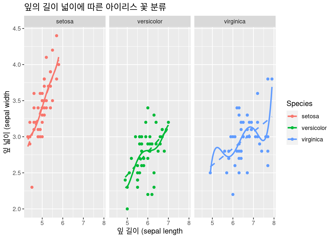

6.2.2.3 geom_bar()

아이리스 꽃 별 갯수를 그려보겠습니다. 50개씩 있네요.

iris %>% # 데이터 선정
  ### 기본 설정 
  ggplot(aes(x = Species,  
             fill = Species)) + # 색 구별 추가!
  xlab("아이리스 종류") + 
  ylab("갯수") +
  ggtitle("아이리스 꽃 별 갯수") +
  geom_bar()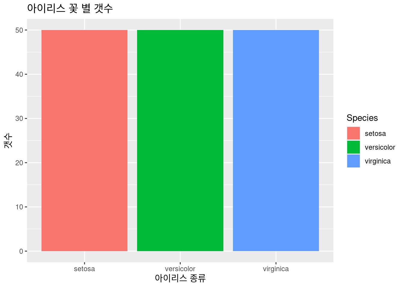

아이리스 꽃 별 갯수를 그려보겠습니다.Sepal.Width 가 3 이상인 것의 갯수를 그려보겠습니다. filter(Sepal.Width > 3)을 이용하겠습니다. 만약 길이가 길다면 아이리스 중에 어떤 종류일까요?

iris %>% 
  filter(Sepal.Width >3) %>%  # 데이터 선정
  
  ### 기본 설정 
  ggplot(aes(x = Species,  
             fill = Species)) + # 색 구별 추가!
  xlab("아이리스 종류 (길이가 3 이상") + 
  ylab("갯수") +
  ggtitle("아이리스 꽃 별 갯수") +
  geom_bar()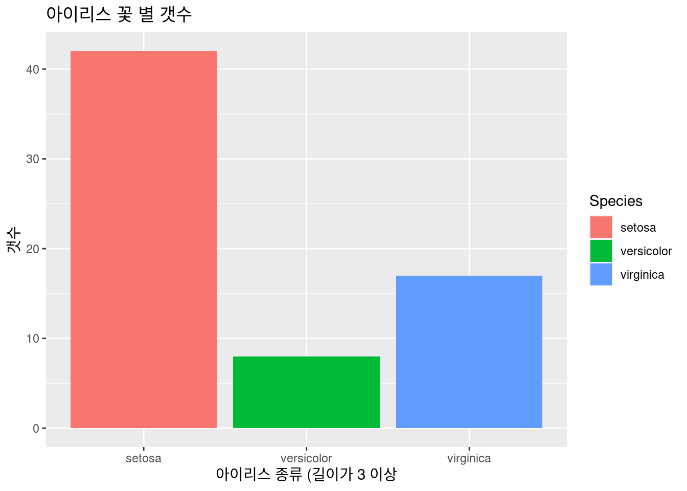

파이 차트 등도 barplot의 하위로 할 수 있

iris %>% 
  filter(Sepal.Width >3) %>%  # 데이터 선정
  
  ### 기본 설정 
  ggplot(aes(x = Species,  
             fill = Species)) + # 색 구별 추가!
  xlab("아이리스 종류 (길이가 3 이상") + 
  ylab("갯수") +
  ggtitle("아이리스 꽃 별 갯수") +
  geom_bar(width =1) + coord_polar()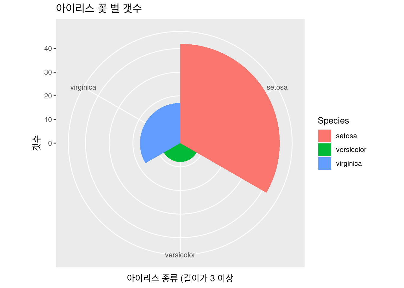

6.2.2.4 geom_density() , geom_histogram()

잎의 넓이의 분포를 그려보겠습니다. histogram과 density를 그려보았습니다.

iris %>% # 데이터 선정
  ### 기본 설정 
  ggplot(aes(x = Sepal.Length)) + # 색 구별 추가!
  xlab("아이리스 잎 넓이") + 
  ylab("밀도") +
  ggtitle("아이리스 잎 넓이 분포") +
  geom_histogram(aes(y = ..density..))+
  geom_density()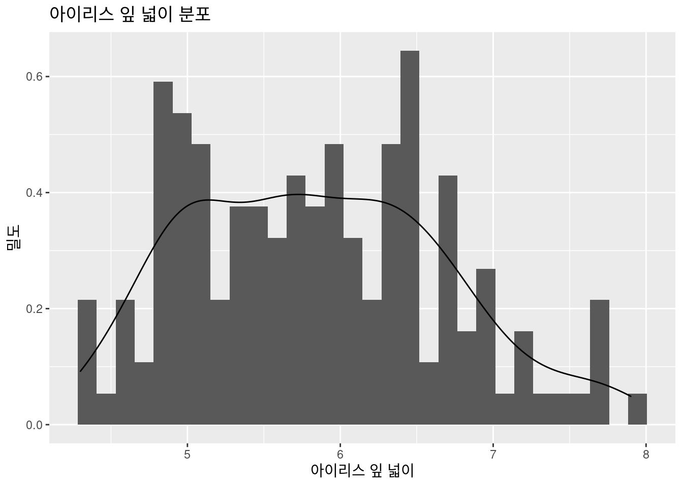

뭔가 어정쩡하게 나왔습니다. heterogeniety 가 보이네요. 안보이신 다고요. aes() 안에 fill = Species를 넣어 구별해 보겠습니다. virginica가 잎이 넓네요. 앞서 했던 color = Species 와 무엇이 다른가요?

iris %>% # 데이터 선정
  ### 기본 설정 
  ggplot(aes(x = Sepal.Length, fill = Species)) + # 색 구별 추가!
  xlab("아이리스 잎 넓이") + 
  ylab("밀도") +
  ggtitle("아이리스 잎 넓이 분포") +
  geom_histogram(aes(y = ..density..), alpha = 0.3)+
  geom_density(stat="density", alpha = 0.3) +
  theme_minimal() # 이거는 제가 좋아하는 테마라 넣어 봤습니다.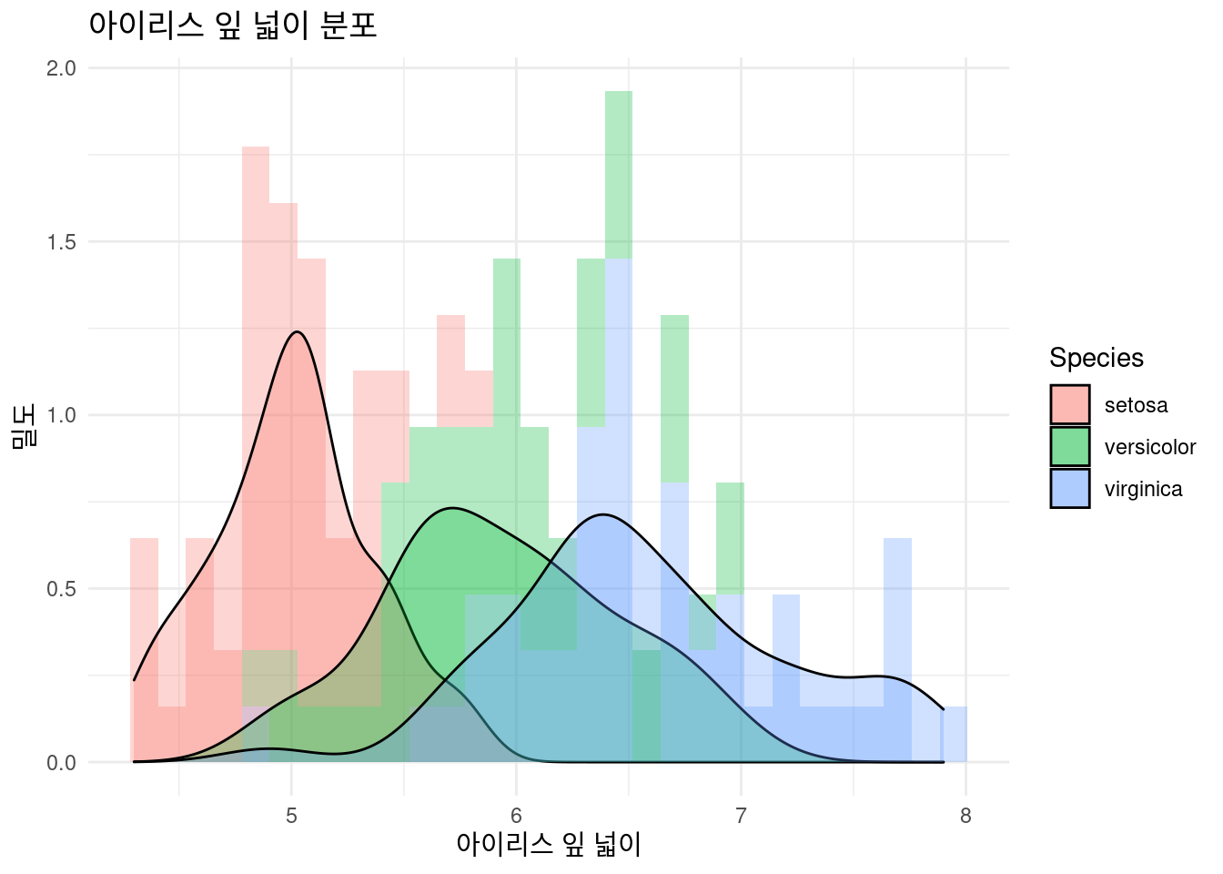 

당연히 faceting을 해볼 수 있습니다. 이런 경우 faceting이 좋은가요? 없는 것이 좋은가요? 연구자 목적 마다 다를 수 있습니다.

iris %>% # 데이터 선정
  ### 기본 설정 
  ggplot(aes(x = Sepal.Length, fill = Species)) + # 색 구별 추가!
  xlab("아이리스 잎 넓이") + 
  ylab("밀도") +
  ggtitle("아이리스 잎 넓이 분포") +
  geom_histogram(aes(y = ..density..), alpha = 0.3)+
  geom_density(stat="density", alpha = 0.3) +
  theme_minimal() + # 이거는 제가 좋아하는 테마라 넣어 봤습니다. 
  facet_wrap(Species~.)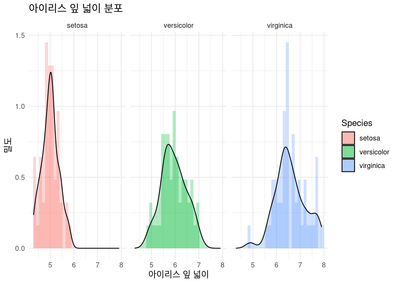

6.2.2.5 geom_boxplot()

아이리스 꽃 별 잎의 넓이 분포를 boxplot을 그려보겠습니다.

iris %>% # 데이터 선정
  ### 기본 설정 
  ggplot(aes(x = Species, y = Sepal.Width, 
             color = Species)) + # 색 구별 추가!
  xlab("아이리스 종류") + 
  ylab("잎 넓이 (sepal width)") +
  ggtitle("아이리스 꽃 별 잎의 넓이 분포") +
  geom_boxplot()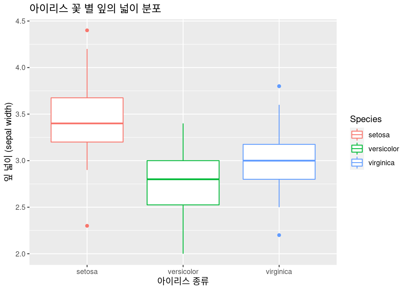

퀴즈! 아이리스 꽃 별 잎의 넓이 분포를 boxplot을 그려보겠습니다.

iris %>% # 데이터 선정
  ### 기본 설정 
  ggplot(aes(x = Species, y = Sepal.Length, 
             color = Species)) + # 색 구별 추가!
  xlab("아이리스 종류") + 
  ylab("잎 길이 (sepal length)") +
  ggtitle("아이리스 꽃 별 잎의 길이 분포") +
  geom_boxplot()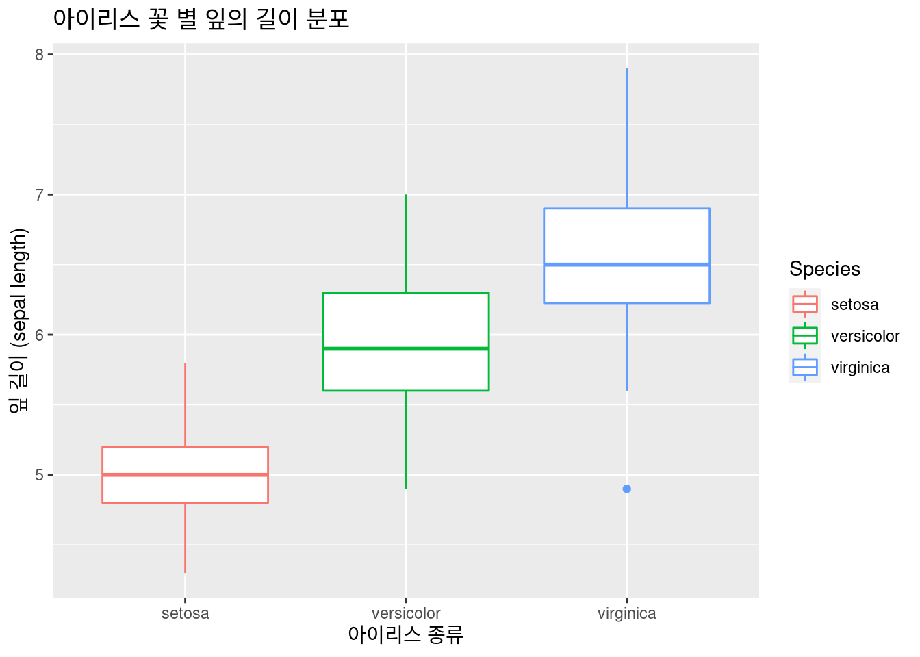

#### 3d plot

지금 까지의 실습을 보면 잎의 넓이과 길이에 따라 종류가 구별될수 있을 것 같은데요, 이때 3d plot을 그려보면서 알아볼 수 있을 것 같습니다. plot_ly는 ggplot 보다 상호 작용 부분과 3d 부분에서 더 우수합니다. 기본적인 것은 ggplot을 실습하시고 필요할 때 plotly를 사용하면 될 것 같습니다. 이번에는 3d plot을 위해서.. 해보겠습니다.

library(plotly)
iris %>%
plot_ly(  # Data
        x = ~Sepal.Length, y = ~Petal.Length, z = ~Petal.Width,  
        color = ~Species,  # Color separation by Species. 
        type = "scatter3d",   # 3d plot을 그린다는 의미
         alpha = 0.8
        ) %>%  
        layout(
               scene = list(xaxis = list(title = '꽃 받침 길이'), 
                            yaxis = list(title = '꽃 잎 길이'),
                            zaxis = list(title = '꽃 잎 넓이')))

6.2.2.6 simple machine learning decision tree

즉 잎과 꽃 바침의 길이 넓이에 따라 Decision tree를 만들수도 있을 것 같다는 생각이 드시죠? 여기까지 왔으니, 간단한 예제로 플로우만 보도록 하겠습니다.

6.2.2.6.1 데이터를 7:3으로 training과 test를 나눕니다.

library(caret) # caret package 불러오기
data(iris)
set.seed(2020)
train_index <- createDataPartition(
           y= iris$Species,  # 종속변수 
           p = .7,  # 70% vs 30%.으로 나누기
           list = FALSE,
           times = 1)  # 중복 없이
train_data <- iris[ train_index,]  # train 데이터 만들기
test_data  <- iris[-train_index,]  # test 데이터 만들기

6.2.2.6.2 10 fold cross validation

cross validation 개발

fitControl <- trainControl(method = "cv", # cross validation
                           number = 10    ) # 10번

6.2.2.6.3 machine learning 모델

모델 개발,결과 보기 94% 정확도.

DTFit1 <- train(data = train_data, # train data를 이용하라
                
                Species ~ ., # . 은 모든 변수를 다 이용하라
                method = 'rpart', # https://topepo.github.io/caret/available-models.html 여기서 찾아 보세요
               trControl = fitControl) # 아까 만든 cross validation
confusionMatrix(DTFit1) # 결과 보기

## Cross-Validated (10 fold) Confusion Matrix 
## 
## (entries are percentual average cell counts across resamples)
##  
##             Reference
## Prediction   setosa versicolor virginica
##   setosa       33.3        0.0       0.0
##   versicolor    0.0       30.5       1.9
##   virginica     0.0        2.9      31.4
##                             
##  Accuracy (average) : 0.9524

그럼 무엇이 관련이 있는가

6.2.2.6.4 barplot for importance

그런 예측을 하는데 중요도가 변수 만다 다릅니다. 이것을 importance라고 합니다 이것 bar plot으로 그려보겠습니다 .

fit1_imp <- varImp(DTFit1)
fit1_imp %>% 
ggplot(mapping = aes(x = Overall)) + 
  geom_boxplot() + 
  labs(title = "Decision Tree에서 변수별 중요도") 

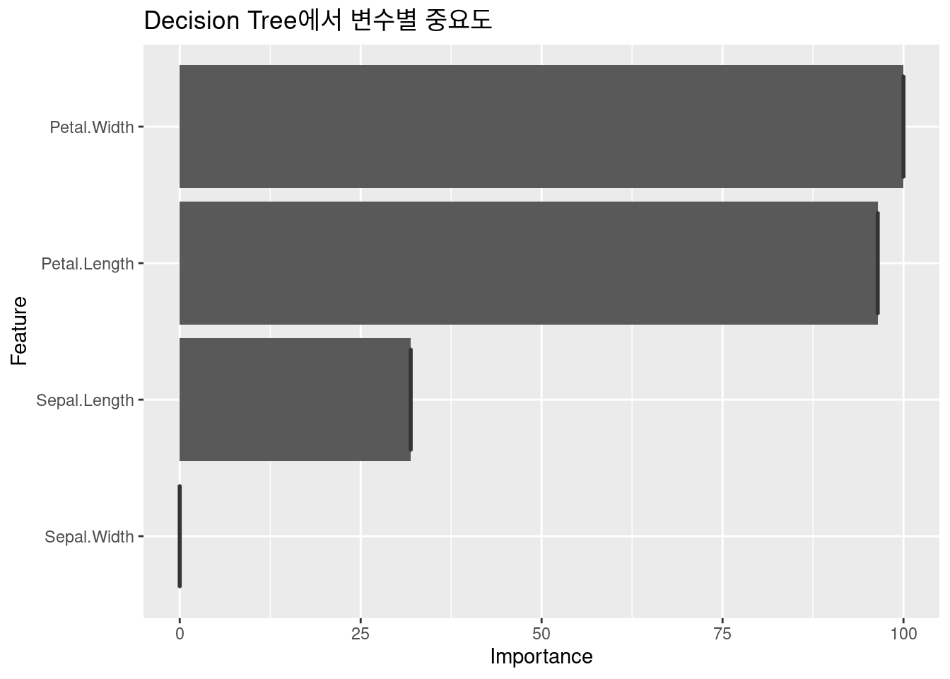##### decision tree ploting

이것을 그림으로 그려 보면 다음과 같습니다.

library(rpart)
library(rattle)
fancyRpartPlot(DTFit1$finalModel)

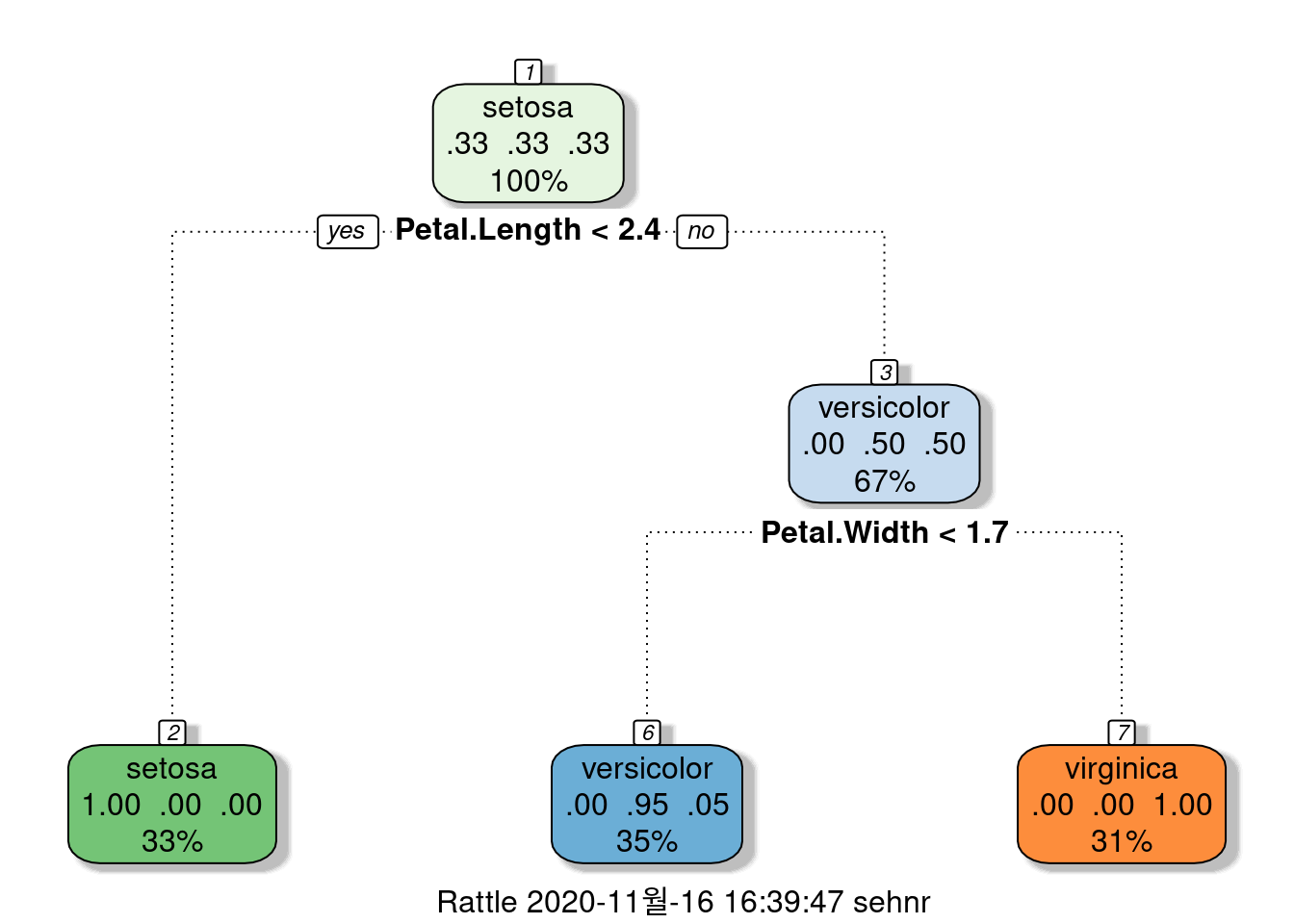
6.3 보건학에서 주로 사용하는 표

아래의 글들과 함께 동영상도 같이 시청하면서 공부하시면 편할 것 같습니다.

동영상	링크
1번	https://youtu.be/6zcM-Zq660E
1번
2번	https://youtu.be/Bhph6EQcPzA
2번
3번	https://youtu.be/5pjBRkIKSN4
3번
4번	https://youtu.be/r9lAGY5C6A4
4번
5번	https://youtu.be/BYNlxRFyHOQ
5번

6.3.1 표1, 또는 기초 그래프

표1은 데이터의 분포를 나타내고, 연속변수인 경우 평균과 표준편차, 또는 중간값과 25%-95% 값을 나타냅니다. 명목변수인 경우에는 빈도와 백분율 등으로 나타냅니다. 우선 15 ~ 65세의 연령에 남녀가 있는 경우를 예로 들겠습니다.

n = 100
age <- sample(c(15:65), n, replace = TRUE)
hist(age)

gender <- sample(c('Women', 'Men'), n, replace = TRUE)
table(gender) %>%
  pie()

group <- sample(c('A', 'B'), n, replace = TRUE)
table(group) %>%
  pie()

dat <- data.frame(age, gender, group)

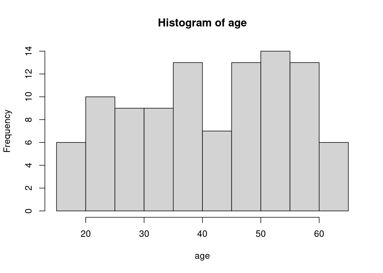
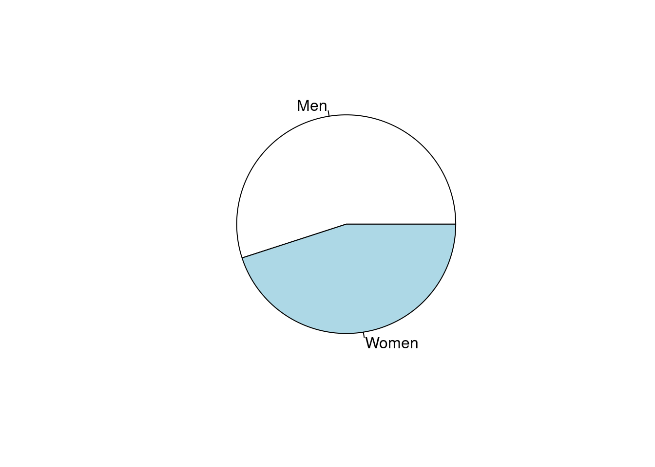
평균 표준편차, 중간값 25%, 75% 순위값으로 연령을, 명수 (%)로 성별을 나타내 보겠습니다. 기본적인 함수는 아래와 같습니다 .

mean(age) # 평균

## [1] 41.73

sd(age) # 표준편차

## [1] 13.69277

median(age) # 중앙값

## [1] 42

quantile(age, probs=c(0.25, 0.75)) # 25%, 75% 값

##   25%   75% 
## 30.75 52.25

table(gender) # 명수

## gender
##   Men Women 
##    55    45

CrossTable(gender) # 백분율과 함께

## 
##  
##    Cell Contents
## |-------------------------|
## |                       N |
## |         N / Table Total |
## |-------------------------|
## 
##  
## Total Observations in Table:  100 
## 
##  
##           |       Men |     Women | 
##           |-----------|-----------|
##           |        55 |        45 | 
##           |     0.550 |     0.450 | 
##           |-----------|-----------|
## 
## 
## 
## 

CrossTable(group, gender) # 집단에 따른 분율

## 
##  
##    Cell Contents
## |-------------------------|
## |                       N |
## | Chi-square contribution |
## |           N / Row Total |
## |           N / Col Total |
## |         N / Table Total |
## |-------------------------|
## 
##  
## Total Observations in Table:  100 
## 
##  
##              | gender 
##        group |       Men |     Women | Row Total | 
## -------------|-----------|-----------|-----------|
##            A |        26 |        26 |        52 | 
##              |     0.236 |     0.289 |           | 
##              |     0.500 |     0.500 |     0.520 | 
##              |     0.473 |     0.578 |           | 
##              |     0.260 |     0.260 |           | 
## -------------|-----------|-----------|-----------|
##            B |        29 |        19 |        48 | 
##              |     0.256 |     0.313 |           | 
##              |     0.604 |     0.396 |     0.480 | 
##              |     0.527 |     0.422 |           | 
##              |     0.290 |     0.190 |           | 
## -------------|-----------|-----------|-----------|
## Column Total |        55 |        45 |       100 | 
##              |     0.550 |     0.450 |           | 
## -------------|-----------|-----------|-----------|
## 
## 

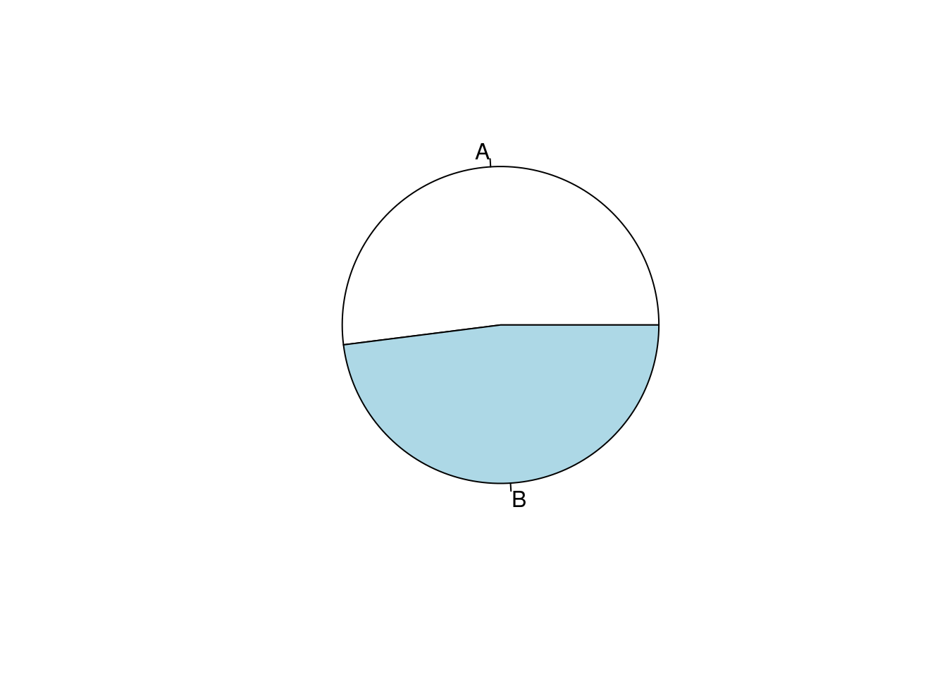
물론 tidyverse 를 이용하여 분석하는 것이 더 편리합니다. 특히 집단별 비교라던가 하는 조건등이 있을때 편리합니다.집단(A, B)에 따른 상기 값을 구해보겠습니다 .

dat %>%
  group_by(group) %>%
  summarise(age_mean = mean(age), 
            age_std   = sd (age))

## # A tibble: 2 x 3
##   group age_mean age_std
##   <chr>    <dbl>   <dbl>
## 1 A         41.0    13.9
## 2 B         42.5    13.6

dat %>%
  group_by(group) %>%
  count(gender) # 성별 명수만 나타냄

## # A tibble: 4 x 3
## # Groups:   group [2]
##   group gender     n
##   <chr> <chr>  <int>
## 1 A     Men       26
## 2 A     Women     26
## 3 B     Men       29
## 4 B     Women     19

dat %>%
  group_by(group) %>%
  count(gender) %>%
  mutate(prob = n/sum(n)) # 성별 명수와 분율 표시

## # A tibble: 4 x 4
## # Groups:   group [2]
##   group gender     n  prob
##   <chr> <chr>  <int> <dbl>
## 1 A     Men       26 0.5  
## 2 A     Women     26 0.5  
## 3 B     Men       29 0.604
## 4 B     Women     19 0.396

표를 만들때 변수가 매우 많을 경우 반복작업을 많이 하게됩니다. 자료의 분포를 보고 의미를 찾아내는 것을 위해 너무 많은 시간과 반복 작업을 하게된다는 것입니다. 특히 소통을 위해 기본 표를 만드는 것에 상당 시간이 걸리게 됩니다. 상급자와 연구를 같이 진행하면서, 표를 만들어 간 후 방법이 바뀔 때마다 얼마나 많은 엑셀과 워드 작업을 했었나요? 가장 지치는 작업중 하나입니다. 다행히 R library 중에 Table 1 등 여러 라이브러리가 이러한 반복 작업을 줄여줄 수 있습니다. 저번 시간에 만든 근로환경조사 데이터를 이용하여 실습하겠습니다. 저번 실습 및 과제때 만든 데이터 과정을 아래에 수록했습니다.

a=read_sas("data/kwcs5th.sas7bdat") # 근로환경조사 5차
# 변수생성: 온콜 여부/빈도, 우울, 연령, 성별, 교육, 근무시간, 종사상지위, 고용형태, 소득#
a0<-a %>%
    select(Q35, AGE, TSEX, TEF1, Q22_1, Q05, Q06, EF11, EF12, Q69,Q62_1_8, Q35) 
# 변수 구획 정하기 ------

Wh_breaks <- c(-Inf, 35, 45, 55, 65, Inf)
Wh_labels <- c('<35','35-44','45-54','55-64','>=65')
inc_break <- c(-Inf, 100, 200, 300, 400, Inf)
inc_label <- c('<100', '100-199', '200-299', '300-399', '>400')

# 데이터 step ------
a1 <-a0 %>%
   filter(AGE <65 ) %>% #50205 --> 41807 : 8401명 제외
   filter(!is.na(Q22_1)) %>% 
   filter(!TEF1    == 9) %>%
   filter(!Q69     == 9) %>%
   filter(!Q62_1_8 == 9) %>% # 41807 --> 41589 :218 명 제외
   mutate(oncall    = Q35) %>%
   mutate(oncallgp  = ifelse(oncall %in% c(1, 2, 3), "on call", "non-on call")) %>%
   mutate(oncallgp3 = ifelse(oncall %in% c(1,2,3), "several times a month", 
                      ifelse(oncall %in% c(4), "rarely", "none"))) %>%
   mutate(oncallgp3 = factor(oncallgp3, 
                         levels=c("none", "rarely", "several times a month")))%>%
   mutate(agegp     = ifelse(AGE <30, '<30', 
                             ifelse(AGE <40, '30-49', 
                                    ifelse(AGE <50, '40-49', 
                                           ifelse(AGE < 60, '50-59', '≥60'))))) %>%
   mutate(Wh=cut(Q22_1, breaks=Wh_breaks, include.lowest=TRUE, right=FALSE, 
                        labels=Wh_labels)) %>% 
   mutate(Wh=structure(Wh, label='Working hours')) %>%
   mutate(Gender=factor(TSEX, levels=c(1,2), labels=c('Men', 'Women') )) %>%
   mutate(Education=factor(TEF1, levels=c(1,2,3,4), 
                        labels=(c('Primary', 'Middle', 'High', 'University')))) %>%
   mutate(Statusw=ifelse(Q05 %in% c(1,2), 'Self employer', 
                         ifelse(Q05 %in% c(3), 'Paid worker', 
                                'Family workers and others'))) %>%
   mutate(inc1=ifelse(EF11 <10000, EF11, ifelse(EF12<10, EF12*100-50, NA) )) %>%
   mutate(inc=cut(inc1, breaks=inc_break, labels=inc_label)) %>%
   mutate(job_st = factor(Q69, levels = c(1:4), 
                  labels = c("Very satisfied", "Satisfied", "Unsatisfied", "Very unsatisfied"))) %>%
   mutate(job_st = structure(job_st, label = 'Job Satisfaction')) %>%
   mutate(depression = Q62_1_8)%>%
   mutate(depression = structure(factor(depression, levels=c(1, 2), 
                                     labels=c("Depression", "Non depression"))))

이때 온콜과 연령에 대한 표를 만들겠습니다. cat.varlist 뒤에는 명목변수를, cont.varlist에는 연속변수를 넣습니다. cat.rmstat, cont.rmstat에는 표시하지 않을 항목을 넣습니다. 마지막 htmlTable()은 이것을 html에 출력해서 복사 붙여 넣기가 쉽게 되도록 하는 것입니다.

make.table(dat =a1,
           cat.varlist  = c("oncallgp"), # 명목변수
           cat.rmstat   = list(c("col")), #
           cont.varlist = c("AGE"), # 연속변수
           cont.rmstat  = list(c("count"))) %>% htmlTable()

##         Variable        Overall
##  AGE                           
##     Mean (SD)     46.29 (11.09)
##     Median (IQR)  48.00 (17.00)
##     Q1, Q3            38.00, 55
##     Min, Max          17.00, 64
##     Missing                   0
##                                
##  oncallgp                      
##    Count                  41589
##    (%)                         
##    non-on call   39818 (95.74%)
##    on call        1771 ( 4.26%)
##    Missing                    0
## 

	Variable	Overall
1	AGE
2	Mean (SD)	46.29 (11.09)
3	Median (IQR)	48.00 (17.00)
4	Q1, Q3	38.00, 55
5	Min, Max	17.00, 64
6	Missing	0
7
8	oncallgp
9	Count	41589
10	(%)
11	non-on call	39818 (95.74%)
12	on call	1771 ( 4.26%)
13	Missing	0
14

6.3.2 종속변수를 중심으로한 표 1 만들기

보건학에서 가장 자주 사용하는 표는, 종속변수를 맨 위에 넣고 관심변수의 분포를 보여주는 것입니다. 위에 Table 1 라이브러리에서 strat라는 항목이있는데, 이는 tidy에서 group_by에 해당한다고 보시면 됩니다. strat에 종속변수 (depression) 을 넣고 표를 만들어 보겠습니다.

tb1<-make.table(dat          = a1,
                strat        = c("depression"),
                cat.varlist  = c("oncallgp", "agegp", "Gender", "Education", "Wh", 
                                 'inc'),
                #"job_st",
                cat.rmstat   = list(c("count", "col", "miss")),
                cat.ptype    = c("chisq"),
                
                cont.varlist = c("AGE"),
                cont.rmstat  = list(c("count","miss", "minmax", "q1q3", "mediqr")),
                cont.ptype   = c( "ttest"))

##         Variable    Depression Non.depression         Overall    p.value
##  AGE                                                              <0.001
##     Mean (SD)    48.69 (10.68)  46.23 (11.10)   46.29 (11.09)     t-test
##                                                                         
##  oncallgp                                                         <0.001
##    (Row %)                                                    Chi-square
##    non-on call    937 ( 2.35%) 38881 (97.65%) 39818 (100.00%)           
##    on call         69 ( 3.90%)  1702 (96.10%)  1771 (100.00%)           
##                                                                         
##  agegp                                                            <0.001
##    (Row %)                                                    Chi-square
##    <30             65 ( 1.69%)  3771 (98.31%)  3836 (100.00%)           
##    ≥60           178 ( 3.47%)  4954 (96.53%)  5132 (100.00%)           
##    30-49          145 ( 1.80%)  7898 (98.20%)  8043 (100.00%)           
##    40-49          265 ( 2.32%) 11136 (97.68%) 11401 (100.00%)           
##    50-59          353 ( 2.68%) 12824 (97.32%) 13177 (100.00%)           
##                                                                         
##  Wh                                                               <0.001
##    (Row %)                                                    Chi-square
##    <35            125 ( 3.06%)  3957 (96.94%)  4082 (100.00%)           
##    35-44          317 ( 1.96%) 15854 (98.04%) 16171 (100.00%)           
##    45-54          263 ( 2.21%) 11656 (97.79%) 11919 (100.00%)           
##    55-64          162 ( 2.56%)  6154 (97.44%)  6316 (100.00%)           
##    >=65           139 ( 4.48%)  2962 (95.52%)  3101 (100.00%)           
##                                                                         
##  Gender                                                           <0.001
##    (Row %)                                                    Chi-square
##    Men            408 ( 2.07%) 19346 (97.93%) 19754 (100.00%)           
##    Women          598 ( 2.74%) 21237 (97.26%) 21835 (100.00%)           
##                                                                         
##  Education                                                        <0.001
##    (Row %)                                                    Chi-square
##    Primary         46 ( 5.38%)   809 (94.62%)   855 (100.00%)           
##    Middle         101 ( 3.91%)  2481 (96.09%)  2582 (100.00%)           
##    High           439 ( 2.53%) 16892 (97.47%) 17331 (100.00%)           
##    University     420 ( 2.02%) 20401 (97.98%) 20821 (100.00%)           
##                                                                         
##  inc                                                              <0.001
##    (Row %)                                                    Chi-square
##    <100           119 ( 3.50%)  3278 (96.50%)  3397 (100.00%)           
##    100-199        379 ( 2.69%) 13719 (97.31%) 14098 (100.00%)           
##    200-299        244 ( 1.97%) 12148 (98.03%) 12392 (100.00%)           
##    300-399        109 ( 1.73%)  6179 (98.27%)  6288 (100.00%)           
##    >400           126 ( 2.79%)  4397 (97.21%)  4523 (100.00%)           
## 

rownames(tb1) <- c()
tb1 %>% htmlTable()

	Variable	Depression	Non.depression	Overall	p.value
1	AGE				<0.001
2	Mean (SD)	48.69 (10.68)	46.23 (11.10)	46.29 (11.09)	t-test
3
4	oncallgp				<0.001
5	(Row %)				Chi-square
6	non-on call	937 ( 2.35%)	38881 (97.65%)	39818 (100.00%)
7	on call	69 ( 3.90%)	1702 (96.10%)	1771 (100.00%)
8
9	agegp				<0.001
10	(Row %)				Chi-square
11	<30	65 ( 1.69%)	3771 (98.31%)	3836 (100.00%)
12	≥60	178 ( 3.47%)	4954 (96.53%)	5132 (100.00%)
13	30-49	145 ( 1.80%)	7898 (98.20%)	8043 (100.00%)
14	40-49	265 ( 2.32%)	11136 (97.68%)	11401 (100.00%)
15	50-59	353 ( 2.68%)	12824 (97.32%)	13177 (100.00%)
16
17	Wh				<0.001
18	(Row %)				Chi-square
19	<35	125 ( 3.06%)	3957 (96.94%)	4082 (100.00%)
20	35-44	317 ( 1.96%)	15854 (98.04%)	16171 (100.00%)
21	45-54	263 ( 2.21%)	11656 (97.79%)	11919 (100.00%)
22	55-64	162 ( 2.56%)	6154 (97.44%)	6316 (100.00%)
23	=65	139 ( 4.48%)	2962 (95.52%)	3101 (100.00%)
24
25	Gender				<0.001
26	(Row %)				Chi-square
27	Men	408 ( 2.07%)	19346 (97.93%)	19754 (100.00%)
28	Women	598 ( 2.74%)	21237 (97.26%)	21835 (100.00%)
29
30	Education				<0.001
31	(Row %)				Chi-square
32	Primary	46 ( 5.38%)	809 (94.62%)	855 (100.00%)
33	Middle	101 ( 3.91%)	2481 (96.09%)	2582 (100.00%)
34	High	439 ( 2.53%)	16892 (97.47%)	17331 (100.00%)
35	University	420 ( 2.02%)	20401 (97.98%)	20821 (100.00%)
36
37	inc				<0.001
38	(Row %)				Chi-square
39	<100	119 ( 3.50%)	3278 (96.50%)	3397 (100.00%)
40	100-199	379 ( 2.69%)	13719 (97.31%)	14098 (100.00%)
41	200-299	244 ( 1.97%)	12148 (98.03%)	12392 (100.00%)
42	300-399	109 ( 1.73%)	6179 (98.27%)	6288 (100.00%)
43	400	126 ( 2.79%)	4397 (97.21%)	4523 (100.00%)
44

6.3.3 관심변수를 중심으로 한 표 2 만들기

이번에는 온콜 여부에 따라 관심변수의 분포를 확인해 보겠습니다. 이는 보건학 연구방법론이나 역학적 연구방법론에서 보정할 변수 또는 층화할 변수 등 향후 분석방법에 대한 방향 설정에 중요하게 다루어집니다. 본 수업에서는 자세한 설명은 하지 않겠습니다.

 tb2<-make.table(dat          = a1,
                 strat        = c("oncallgp3"),
                 cat.varlist  = c("agegp", "Gender", "Education", "Wh", 
                                  'inc','depression'),
                 #,"job_st"
                 cat.rmstat   = list(c("count", "col", "miss")),
                 cat.ptype    = c("chisq"),
                 cont.varlist = c("AGE"),
                 cont.rmstat  = list(c("count","miss", "minmax", "q1q3", "mediqr")),
                 cont.ptype   = c( "anova"))

##          Variable           none        rarely several.times.a.month
##  AGE                                                                
##     Mean (SD)      46.53 (11.10) 44.82 (10.99)         46.41 (10.97)
##                                                                     
##  agegp                                                              
##    (Row %)                                                          
##    <30             3062 (79.82%)  620 (16.16%)          154 ( 4.01%)
##    ≥60            4414 (86.01%)  514 (10.02%)          204 ( 3.98%)
##    30-49           6378 (79.30%) 1320 (16.41%)          345 ( 4.29%)
##    40-49           9294 (81.52%) 1624 (14.24%)          483 ( 4.24%)
##    50-59          10869 (82.48%) 1723 (13.08%)          585 ( 4.44%)
##                                                                     
##  Wh                                                                 
##    (Row %)                                                          
##    <35             3419 (83.76%)  434 (10.63%)          229 ( 5.61%)
##    35-44          13013 (80.47%) 2544 (15.73%)          614 ( 3.80%)
##    45-54           9492 (79.64%) 1835 (15.40%)          592 ( 4.97%)
##    55-64           5397 (85.45%)  703 (11.13%)          216 ( 3.42%)
##    >=65            2696 (86.94%)  285 ( 9.19%)          120 ( 3.87%)
##                                                                     
##  Gender                                                             
##    (Row %)                                                          
##    Men            15392 (77.92%) 3448 (17.45%)          914 ( 4.63%)
##    Women          18625 (85.30%) 2353 (10.78%)          857 ( 3.92%)
##                                                                     
##  Education                                                          
##    (Row %)                                                          
##    Primary          774 (90.53%)   60 ( 7.02%)           21 ( 2.46%)
##    Middle          2239 (86.72%)  244 ( 9.45%)           99 ( 3.83%)
##    High           14372 (82.93%) 2232 (12.88%)          727 ( 4.19%)
##    University     16632 (79.88%) 3265 (15.68%)          924 ( 4.44%)
##                                                                     
##  inc                                                                
##    (Row %)                                                          
##    <100            2932 (86.31%)  347 (10.21%)          118 ( 3.47%)
##    100-199        11894 (84.37%) 1640 (11.63%)          564 ( 4.00%)
##    200-299         9970 (80.46%) 1825 (14.73%)          597 ( 4.82%)
##    300-399         4889 (77.75%) 1121 (17.83%)          278 ( 4.42%)
##    >400            3570 (78.93%)  758 (16.76%)          195 ( 4.31%)
##                                                                     
##  depression                                                         
##    (Row %)                                                          
##    Depression       773 (76.84%)  164 (16.30%)           69 ( 6.86%)
##    Non depression 33244 (81.92%) 5637 (13.89%)         1702 ( 4.19%)
##                                                                     
##          Overall     p.value
##                       <0.001
##    46.29 (11.09) 1-way ANOVA
##                             
##                       <0.001
##                   Chi-square
##   3836 (100.00%)            
##   5132 (100.00%)            
##   8043 (100.00%)            
##  11401 (100.00%)            
##  13177 (100.00%)            
##                             
##                       <0.001
##                   Chi-square
##   4082 (100.00%)            
##  16171 (100.00%)            
##  11919 (100.00%)            
##   6316 (100.00%)            
##   3101 (100.00%)            
##                             
##                       <0.001
##                   Chi-square
##  19754 (100.00%)            
##  21835 (100.00%)            
##                             
##                       <0.001
##                   Chi-square
##    855 (100.00%)            
##   2582 (100.00%)            
##  17331 (100.00%)            
##  20821 (100.00%)            
##                             
##                       <0.001
##                   Chi-square
##   3397 (100.00%)            
##  14098 (100.00%)            
##  12392 (100.00%)            
##   6288 (100.00%)            
##   4523 (100.00%)            
##                             
##                       <0.001
##                   Chi-square
##   1006 (100.00%)            
##  40583 (100.00%)            
## 

rownames(tb2) <- c()
tb2 %>% htmlTable()

	Variable	none	rarely	several.times.a.month	Overall	p.value
1	AGE					<0.001
2	Mean (SD)	46.53 (11.10)	44.82 (10.99)	46.41 (10.97)	46.29 (11.09)	1-way ANOVA
3
4	agegp					<0.001
5	(Row %)					Chi-square
6	<30	3062 (79.82%)	620 (16.16%)	154 ( 4.01%)	3836 (100.00%)
7	≥60	4414 (86.01%)	514 (10.02%)	204 ( 3.98%)	5132 (100.00%)
8	30-49	6378 (79.30%)	1320 (16.41%)	345 ( 4.29%)	8043 (100.00%)
9	40-49	9294 (81.52%)	1624 (14.24%)	483 ( 4.24%)	11401 (100.00%)
10	50-59	10869 (82.48%)	1723 (13.08%)	585 ( 4.44%)	13177 (100.00%)
11
12	Wh					<0.001
13	(Row %)					Chi-square
14	<35	3419 (83.76%)	434 (10.63%)	229 ( 5.61%)	4082 (100.00%)
15	35-44	13013 (80.47%)	2544 (15.73%)	614 ( 3.80%)	16171 (100.00%)
16	45-54	9492 (79.64%)	1835 (15.40%)	592 ( 4.97%)	11919 (100.00%)
17	55-64	5397 (85.45%)	703 (11.13%)	216 ( 3.42%)	6316 (100.00%)
18	=65	2696 (86.94%)	285 ( 9.19%)	120 ( 3.87%)	3101 (100.00%)
19
20	Gender					<0.001
21	(Row %)					Chi-square
22	Men	15392 (77.92%)	3448 (17.45%)	914 ( 4.63%)	19754 (100.00%)
23	Women	18625 (85.30%)	2353 (10.78%)	857 ( 3.92%)	21835 (100.00%)
24
25	Education					<0.001
26	(Row %)					Chi-square
27	Primary	774 (90.53%)	60 ( 7.02%)	21 ( 2.46%)	855 (100.00%)
28	Middle	2239 (86.72%)	244 ( 9.45%)	99 ( 3.83%)	2582 (100.00%)
29	High	14372 (82.93%)	2232 (12.88%)	727 ( 4.19%)	17331 (100.00%)
30	University	16632 (79.88%)	3265 (15.68%)	924 ( 4.44%)	20821 (100.00%)
31
32	inc					<0.001
33	(Row %)					Chi-square
34	<100	2932 (86.31%)	347 (10.21%)	118 ( 3.47%)	3397 (100.00%)
35	100-199	11894 (84.37%)	1640 (11.63%)	564 ( 4.00%)	14098 (100.00%)
36	200-299	9970 (80.46%)	1825 (14.73%)	597 ( 4.82%)	12392 (100.00%)
37	300-399	4889 (77.75%)	1121 (17.83%)	278 ( 4.42%)	6288 (100.00%)
38	400	3570 (78.93%)	758 (16.76%)	195 ( 4.31%)	4523 (100.00%)
39
40	depression					<0.001
41	(Row %)					Chi-square
42	Depression	773 (76.84%)	164 (16.30%)	69 ( 6.86%)	1006 (100.00%)
43	Non depression	33244 (81.92%)	5637 (13.89%)	1702 ( 4.19%)	40583 (100.00%)
44

6.3.4 상관관계를 위한 표 3 만들기

이제 관심변수와 종속변수가 어떠한 상관관계가 있는지 알아보기 위해 가장 많이 사용되는 분석 표를 만들어 보겠습니다. 가장 직관적이고 많이 사용되는 것인 로지스틱회귀 분석이면, 단변령, 다변량으로 나누어 분석합니다. 여기서 기본 인구학적 요소를 보정한 것을 model 2, 이후 모든 변수를 보정한 것을 model 3로 하여 나타내 보도록 하겠습니다. 역시, 로지스틱 회귀분석에 대해서는 보건학연구방법론 등에서 공부하시기를 바랍니다. 아래는 보정 없는 모델부터 모두 보정한 모델까지 fit1.1, fit1.2, fit1.3로 만들었고 이에 summary 함수에 따라 베타 값과 p value가 나타나게 됩니다. 이때 베타 값에 exp()를 한 값이 오즈비가 됩니다. 여기에 95% 신뢰구간을 수록하여 표 3을 만들게 됩니다.

a1 <- a1 %>%
  mutate(oncallgp = factor(oncallgp)) %>%
  mutate(Wh = relevel(Wh, ref = '35-44'))
fit1.1 <- glm(data=a1, family=binomial, #로지스틱회귀분석 돌린다는 이야기 OR
              depression=='Depression' ~ oncallgp)
summary(fit1.1) # Estimate (기울기), pr <0.05

## 
## Call:
## glm(formula = depression == "Depression" ~ oncallgp, family = binomial, 
##     data = a1)
## 
## Deviance Residuals: 
##     Min       1Q   Median       3Q      Max  
## -0.2819  -0.2182  -0.2182  -0.2182   2.7384  
## 
## Coefficients:
##                 Estimate Std. Error z value Pr(>|z|)    
## (Intercept)     -3.72558    0.03306 -112.69  < 2e-16 ***
## oncallgpon call  0.52012    0.12717    4.09 4.32e-05 ***
## ---
## Signif. codes:  0 '***' 0.001 '**' 0.01 '*' 0.05 '.' 0.1 ' ' 1
## 
## (Dispersion parameter for binomial family taken to be 1)
## 
##     Null deviance: 9475.8  on 41588  degrees of freedom
## Residual deviance: 9461.2  on 41587  degrees of freedom
## AIC: 9465.2
## 
## Number of Fisher Scoring iterations: 6

fit1.2 <- glm(data=a1, family=binomial,
              depression=='Depression' ~ oncallgp + 
                Gender+Education+inc)

#summary(fit1.2)
fit1.3 <- glm(data=a1, family=binomial,
              depression=='Depression' ~ oncallgp +
                Gender+Education+inc+Wh+job_st)

#summary(fit1.3)

95% 신뢰구간을 구하는 방법은 여럿이 있으나 가장 쉬운 방법은 confint.default(model)을 이요하는 것입니다. 여기에도 exp()를 통해 오즈비에 대한 95% 신뢰구간을 구할 수 있습니다.

confint.default(fit1.2)

##                           2.5 %      97.5 %
## (Intercept)         -3.29687112 -2.59267547
## oncallgpon call      0.33029321  0.83072372
## GenderWomen          0.07221021  0.35391011
## EducationMiddle     -0.65302449  0.09455622
## EducationHigh       -0.99526092 -0.33345130
## EducationUniversity -1.18988022 -0.51642275
## inc100-199          -0.37785941  0.04881440
## inc200-299          -0.60272750 -0.13349178
## inc300-399          -0.70036472 -0.13595821
## inc>400             -0.18891863  0.36475111

exp(cbind(OR=coef(fit1.2), confint.default(fit1.2))) %>% htmlTable()

	OR	2.5 %	97.5 %
(Intercept)	0.052613986311375	0.0369987512130006	0.0748195943056818
oncallgpon call	1.78694679986763	1.39137603507923	2.29497906033384
GenderWomen	1.23745909542807	1.07488127618685	1.42462711629881
EducationMiddle	0.756362790639428	0.520469238276144	1.09917095765098
EducationHigh	0.514604769451131	0.369626989696847	0.716446785877419
EducationUniversity	0.426070060085597	0.304257705086851	0.596651105514402
inc100-199	0.848298666786461	0.685326846175062	1.05002544711034
inc200-299	0.692041302591936	0.547316794297159	0.875034659055465
inc300-399	0.65825593306648	0.496404222223775	0.872879105411584
inc>400	1.09189665961181	0.827853867019981	1.44015551870661

이를 반복하는 것도 번거로운 일입니다. 이에 oddstable이라는 함수를 만들어 사용하겠습니다.

oddstable <- function(fit1.1, fit1.2, fit1.3) {
  list1 <-list(fit1.1, fit1.2, fit1.3)
  orci <-function(models) {
    exp(cbind(OR=coef(models), confint.default(models)))
  }
  odds1<-lapply(list1, orci)
  models <- c(rep('model 1', length(odds1[[1]])/3), 
              rep('model 2', length(odds1[[2]])/3), 
              rep('model 3', length(odds1[[3]])/3))
  var<-do.call('rbind', odds1) %>% rownames()
  do.call('rbind', odds1) %>% data.frame() %>% 
    mutate(models = models, var=var) %>% 
    mutate_if(is.numeric, round, 2) %>%
    mutate_all(format, 2) %>%
    mutate(odds=paste0(OR, " (", `X2.5..`, "-", `X97.5..`,") " )) %>%
    select(var, odds, models) %>% 
    group_by(models) %>% mutate(num2 = row_number()) %>% 
    ungroup() %>%
    spread(key=models, value=odds, convert=FALSE) %>% 
    arrange(num2) 
}

oddstable에 모델 1, 2, 3 을 넣고 실행하면 좀더 간편한 표가 나타나게 됩니다. 다만 완성된 표를 위해서는 referece가 되었던 수준을 1로 표시해 주는 것이 선호됩니다.

oddstable(fit1.1, fit1.2, fit1.3)%>% htmlTable()

	var	num2	model 1	model 2	model 3
1	(Intercept)	1	0.02 (0.02-0.03)	0.05 (0.04-0.07)	0.02 (0.01-0.03)
2	oncallgpon call	2	1.68 (1.31-2.16)	1.79 (1.39-2.29)	1.37 (1.06-1.77)
3	GenderWomen	3		1.24 (1.07-1.42)	1.38 (1.20-1.59)
4	EducationMiddle	4		0.76 (0.52-1.10)	0.77 (0.53-1.13)
5	EducationHigh	5		0.51 (0.37-0.72)	0.61 (0.44-0.85)
6	EducationUniversity	6		0.43 (0.30-0.60)	0.65 (0.46-0.92)
7	inc100-199	7		0.85 (0.69-1.05)	0.85 (0.67-1.08)
8	inc200-299	8		0.69 (0.55-0.88)	0.72 (0.56-0.94)
9	inc300-399	9		0.66 (0.50-0.87)	0.70 (0.51-0.95)
10	inc>400	10		1.09 (0.83-1.44)	1.23 (0.91-1.66)
11	Wh<35	11			1.21 (0.96-1.54)
12	Wh45-54	12			1.07 (0.90-1.26)
13	Wh55-64	13			1.17 (0.95-1.43)
14	Wh>=65	14			1.94 (1.57-2.41)
15	job_stSatisfied	15			1.36 (0.86-2.17)
16	job_stUnsatisfied	16			4.13 (2.59-6.59)
17	job_stVery unsatisfied	17			8.49 (5.15-14.02)

6.3.5 Daniel Lüdecke’s work

최근 Daniel Lüdecke가 package를 업데이트 했습니다. 과거 로지스틱 회귀분석의 경우 표를 만들때 여러 모델을 비교하는 것에 문제가 있었던것을 수정해서 내 놓았네요. (ref: https://cran.r-project.org/web/packages/sjPlot/vignettes/tab_model_estimates.html)

library(sjPlot)
library(sjmisc)
library(sjlabelled)

tab_model(fit1.1, fit1.2, fit1.3, 
              df.method = "wald" )

	depression == “Depression”			depression == “Depression”			depression == “Depression”
Predictors	Odds Ratios	CI	p	Odds Ratios	CI	p	Odds Ratios	CI	p
(Intercept)	0.02	0.02 – 0.03	<0.001	0.05	0.04 – 0.07	<0.001	0.02	0.01 – 0.03	<0.001
oncallgp: on call	1.68	1.31 – 2.16	<0.001	1.79	1.39 – 2.29	<0.001	1.37	1.06 – 1.77	0.015
Gender: Women				1.24	1.07 – 1.42	0.003	1.38	1.20 – 1.59	<0.001
Education: Middle				0.76	0.52 – 1.10	0.143	0.77	0.53 – 1.13	0.177
Education: High				0.51	0.37 – 0.72	<0.001	0.61	0.44 – 0.85	0.004
Education: University				0.43	0.30 – 0.60	<0.001	0.65	0.46 – 0.92	0.015
inc: 100-199				0.85	0.69 – 1.05	0.131	0.85	0.67 – 1.08	0.184
inc: 200-299				0.69	0.55 – 0.88	0.002	0.72	0.56 – 0.94	0.015
inc: 300-399				0.66	0.50 – 0.87	0.004	0.70	0.51 – 0.95	0.022
inc: >400				1.09	0.83 – 1.44	0.534	1.23	0.91 – 1.66	0.182
Wh: <35							1.21	0.96 – 1.54	0.111
Wh: 45-54							1.07	0.90 – 1.26	0.461
Wh: 55-64							1.17	0.95 – 1.43	0.134
Wh: >=65							1.94	1.57 – 2.41	<0.001
Job Satisfaction: Satisfied							1.36	0.86 – 2.17	0.188
Job Satisfaction: Unsatisfied							4.13	2.59 – 6.59	<0.001
Job Satisfaction: Very unsatisfied							8.49	5.15 – 14.02	<0.001
Observations	41589			40698			40698
R2 Tjur	0.000			0.003			0.017

몇가지 만 바꿔보겠습니다.

 tab_model(fit1.1, fit1.2, fit1.3, 
          show.reflvl = TRUE, 
          prefix.labels = "varname",
          df.method = "wald" , show.p = FALSE,
          dv.labels = c("Model 1", "Model 2", "Model 3"))

	Model 1		Model 2		Model 3
Predictors	Odds Ratios	CI	Odds Ratios	CI	Odds Ratios	CI
(Intercept)	0.02	0.02 – 0.03	0.05	0.04 – 0.07	0.02	0.01 – 0.03
oncallgp: non-on call	Reference		Reference		Reference
oncallgp: on call	1.68	1.31 – 2.16	1.79	1.39 – 2.29	1.37	1.06 – 1.77
Gender: Men	Reference		Reference		Reference
Gender: Women			1.24	1.07 – 1.42	1.38	1.20 – 1.59
Education: Primary	Reference		Reference		Reference
Education: Middle			0.76	0.52 – 1.10	0.77	0.53 – 1.13
Education: High			0.51	0.37 – 0.72	0.61	0.44 – 0.85
Education: University			0.43	0.30 – 0.60	0.65	0.46 – 0.92
inc: <100	Reference		Reference		Reference
inc: 100-199			0.85	0.69 – 1.05	0.85	0.67 – 1.08
inc: 200-299			0.69	0.55 – 0.88	0.72	0.56 – 0.94
inc: 300-399			0.66	0.50 – 0.87	0.70	0.51 – 0.95
inc: >400			1.09	0.83 – 1.44	1.23	0.91 – 1.66
Wh: 35-44	Reference		Reference		Reference
Wh: <35					1.21	0.96 – 1.54
Wh: 45-54					1.07	0.90 – 1.26
Wh: 55-64					1.17	0.95 – 1.43
Wh: >=65					1.94	1.57 – 2.41
job_st: Very satisfied	Reference		Reference		Reference
job_st: Satisfied					1.36	0.86 – 2.17
job_st: Unsatisfied					4.13	2.59 – 6.59
job_st: Very unsatisfied					8.49	5.15 – 14.02
Observations	41589		40698		40698
R2 Tjur	0.000		0.003		0.017

6.4 과제

과제는 저번 시간에 여러분이 만든 자신만의 데이터에 대해서 표 1, 2, 3을 만드는 것입니다. 이후 이것을 제출해 주시면됩니다. 표의 예시는 아래와 같습니다.

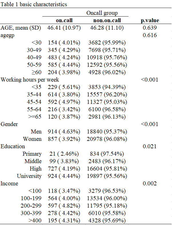
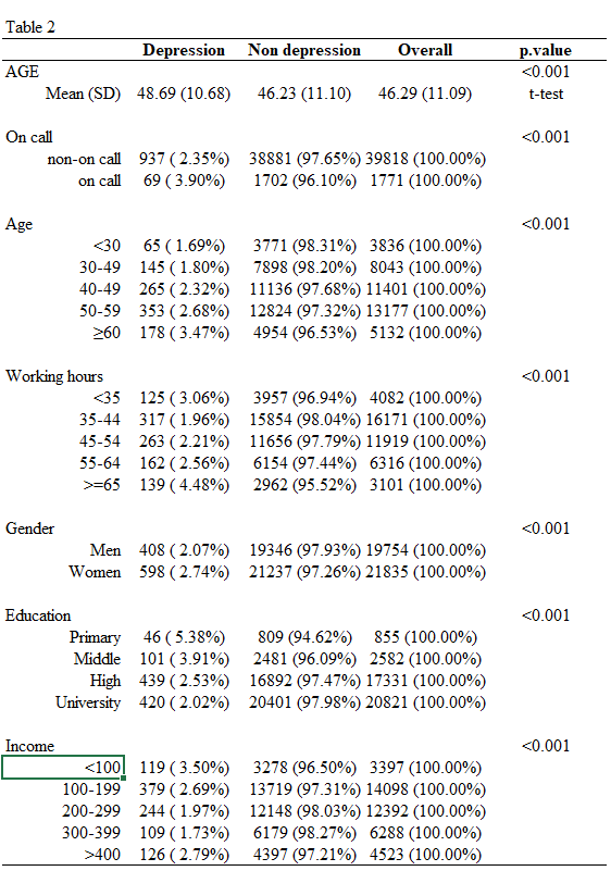
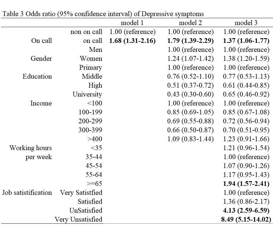
표3