Chapter 8 The Gradient and Linear Approximation

8.1 The Gradient Vector

In one dimension a function is differentiable at a point if we can define the tangent at the point. In two dimesions we need to be able to define the tangent plane at the point. Recalling Taylor series in one dimension in Section 5 we know that the tangent line at a point \((b,f(b))\) is \[ y=f(b)+(x-b)f'(b). \]

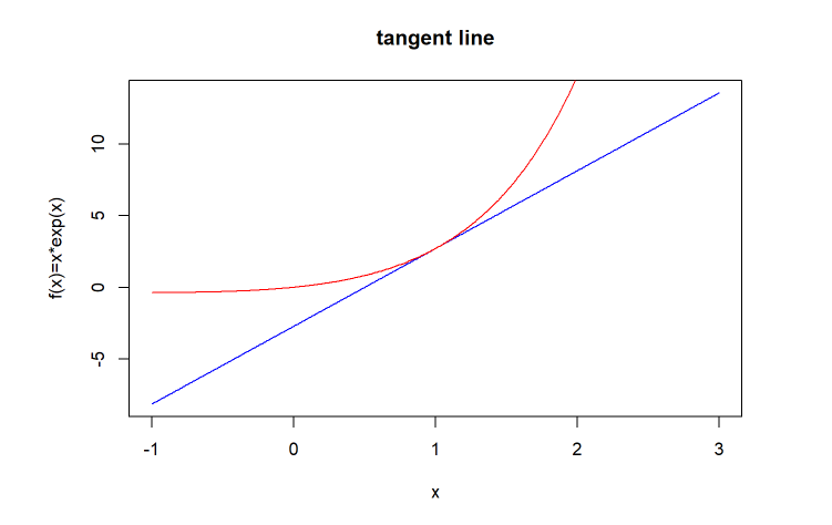
Tangent Line

So how can we generalise the concept of differentiability and the idea of linear approximation, to functions of two variables?

First of all we need to generalise the definition of slope. We do this by introducing the gradient vector. This vector has components which are the slopes on the surface at the point of interest in both directions. In the picture below we look at the tangents to the lines in the surface passing through \((-1/2,1/2)\).

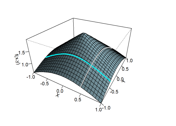
The gradient vector

Definition 8.1 (Gradient Vector) Let \(f\) be a function of two variables with first order partial derivatives. Then the gradient vector \[ \nabla f(x,y) = \left ( {\partial f \over \partial x}, {\partial f \over \partial x} \right ). \]

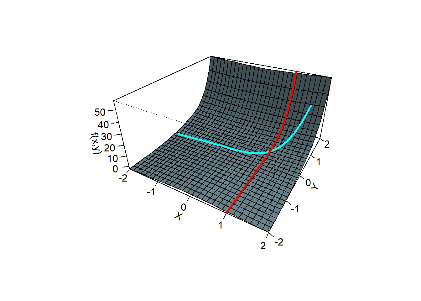
Example 8.1 Find the gradient of the function \(f(x,y)=x \arctan (xy)+\exp(2y)\) at the point \((x,y)=(1,0)\) (see the picture above).

As we see in Example~7.6, \(f_x(1,0)=0\) and \(f_y(1,0)=3\). Hence \[ \nabla f(1,0)=(0,3). \]

Remark. This can be generalised to higher dimensions. Let \(f\) be a function of 3 variables with first order partial derivatives. Then the gradient vector \[ \nabla f (x,y,z) = \left ( {\partial f \over \partial x}, {\partial f \over \partial x}, {\partial f \over \partial z}\right ). \]

Example 8.2 Find the gradient of the function \(f(x,y,z)=x^2y\sin(z)\) at the point \((x,y,z)=(1,2,\pi/3)\).

The first order partial derivatives \[ \nabla f(x,y,x)=(2xy \sin(z), x^2 \sin(z), x^2 y \cos(z)) = (2 \sqrt{3},\sqrt{3},1). \]

8.2 The Directional Derivative

First partial derivatives give the rate of change of a function in the direction of the (positive) \(x\) and \(y\) axes. What about the rate of change in any direction?

Definition 8.2 (Directional Derivative) The directional derivative of a function of several variable \(f\) at \({\bf x}_0\) in the direction of the unit vector (that is a vector of length 1) \({\bf u}\) is given by \[ f_{{\bf u}}({\bf x}_0)=\lim_{h\rightarrow 0}\frac{f({\bf x}_0+h{\bf u})-f({\bf x}_0)}{h}. \]

Directional derivatives are also denoted by: \[ f_{{\bf u}}({\bf x}_0)=\frac{\partial f}{\partial {\bf u}}({\bf x}_0)=D_{{\bf u}}({\bf x}_0). \] They give the rate of change in the direction given by the vector \({\bf u}\), in the same way partial derivatives give the rate of change in the direction of the coordinate axis.

In particular, for bivariate functions, the definition can be written \[ f_{{\bf u}}({\bf x}_0)=\lim_{h\rightarrow 0}\frac{f(x_0+hu,y_0+hv)-f(x_0,y_0)}{h} \] where \({\bf u}=(u,v)\) and \({\bf x}_0=(x_0,y_0)\). From this it is apparent that the partial derivatives are directional derivatives; see Definition 8.2. Indeed \(f_x({\bf x}_0)=f_{{\bf i}}({\bf x}_0)\) and \(f_y({\bf x}_0)=f_{{\bf j}}({\bf x}_0)\).

As usual, we want to avoid the evaluation of a derivative based on its definition. The gradient can be used to calculate directional derivatives, as the following theorem shows.

Theorem 8.1 If \(f\) is differentiable at \({\bf x}\) then the directional derivative of \(f\) at \({\bf x}\) in the direction of the unit vector \({\bf u}\) is given by \[ \tag{8.2} f_{{\bf u}}({\bf x})={\bf u}\cdot \nabla f({\bf x}). \]

Proof: If \(f\) is differentiable, than the composition of function \(f({\bf x}+h{\bf u})\) is a differentiable function of \(h\) and, clearly, \[ \left .f_{{\bf u}}({\bf x})=\frac{df({\bf x}+h{\bf u})}{dh}\right|_{h=0}={\bf u}\cdot \nabla f({\bf x}), \] with the last equality due to Chain Rule I. In Section Challenge Yourself at the end of this chapter you will be asked to give more detail in this proof. \(\Box\)

Example 8.3 Find the rate of change of the function \(f(x,y)=x^3y\) at \({\bf x}_0=(1,-2)\) in the direction \({\bf u}=(1/2,\sqrt{3}/2)\).

The directional derivative \[ f_{{\bf u}}({\bf x}) = {\bf u} \cdot \nabla f ({\bf x}) = (1/2,\sqrt{3}/2) \cdot (3x^2 y, x^3) = (1/2,\sqrt{3}/2) \cdot (-6,1) = -3+\sqrt{3}/2. \]

Remark. In the case where the direction vector \({\bf u}\) is not a unit vector then we have to create a unit vector in the same direction to use in the formula: \({\bf u}/\| {\bf u} \|\). Then we have: \[ f_{{\bf u}/\| {\bf u} \|}({\bf x})=\frac{{\bf u}}{\|{\bf u} \|}\cdot \nabla f({\bf u}). \] So, once again, it is the unit vectors that are relevant. Note that all possible directions (all unit vectors) are given by the vectors pointing at the unit circle, which are given by \[ {\bf u}_\phi=(\cos\phi,\sin\phi)\qquad\phi\in [0,2\pi). \]

This the following example gives a formula to calculate all the directional derivatives.

Example 8.4 Find a formula for the directional derivative of a bivariate function in the direction of the vector \({\bf u}_\phi=(\cos\phi,\sin\phi)\) for \(\phi\in [0,2\pi)\).

Applying Equation (8.2) we get: \[ f_{{\bf u}_\phi}({\bf x}) ={\bf u}_\phi\cdot \nabla f({\bf x})=f_x({\bf x})\cos\phi+f_y({\bf x})\sin\phi. \] In particular, if \(\theta=3\pi/4\), \(f(x,y)=x^2y-xy^2\), and \({\bf x}_0=(2,2)\), we have \[ f_{{\bf u}_\phi}({\bf x}_0) =(-1/\sqrt{2},1\sqrt{2}) \cdot \left . (2xy-y^2,x^2-2xy)\right |_{(2,2)} = (-1/\sqrt{2},1\sqrt{2}) \cdot (4,-4)=-4\sqrt{2}. \]

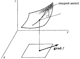
Let \(\theta\) be the angle between \(\nabla f({\bf x})\) and \({\bf u}_\phi\) and assume that \(\nabla f({\bf x})\neq 0\) . Then, \[ f_{{\bf u}_\phi}({\bf x})=\|{\bf u}_\phi\| \|\nabla f({\bf x})\|\cos\theta=\|\nabla f({\bf x})\|\cos\theta. \] (as \(\|{\bf u}_\phi\|=1\)). As \(\cos\theta\) takes values between \(-1\) and \(1\), this implies that \[ -\|\nabla f({\bf x})\|\le f_{{\bf u}_\phi}({\bf x})\le \|\nabla f({\bf x})\|. \] Hence the directional derivative is maximised in the direction of the \(\nabla f\).

From jeffreythompson.org

Also, if \({\bf u}_\phi\) is tangent to the level curve, then \(\cos \theta =0\) and thus \(f_{{\bf u}_\phi}({\bf x})=0\). We can summarize all our findings as follows.

Theorem 8.2 (Geometric properties of the gradient) Let \(f\) be differentiable at \({\bf x}\). Then,

• The gradient of \(f\) at \({\bf x}\) is a vector normal to the level curve (set) passing through \({\bf x}\);
• \(f\) increases most rapidly in the direction of \(\nabla f({\bf x})\);
• \(f\) decreases most rapidly in the direction of \(-\nabla f({\bf x})\);
• the maximum slope (rate of change) of \(f\) at \({\bf x}\) is given by \(\|\nabla f({\bf x})||\);
• the slope (rate of change) of \(f\) is zero in the directions tangent to the level curve of \(f\) passing through \({\bf x}\).

8.2.1 Test yourself

8.3 Tangent planes

A linear approximation to a curve in the \(x-y\) plane is the tangent line. A linear approximation to a surface is three dimensions is a tangent plane, and constructing these planes is an important skill. In the picure below we have an example of the tangent plane to \(z=2-x^2-y^2\), at \((1/2,-1/2)\).

We know that the tangent plane at \((x_0,y_0,f(x_0,y_0))\) has the form \[ z=a(x-x_0)+b(y-y_0)+f(x_0,y_0), \tag{8.1} \] because \(z=f(x_0,y_0)\) at \((x_0,y_0)\). We just need to find out what the coefficients \(a\) and \(b\) are. Now, because the plane is tangent to the surface, the partial derivatives \[ {\partial z \over \partial x}(x_0,y_0) = {\partial f \over \partial x}(x_0,y_0) \quad {\rm and} \quad {\partial z \over \partial y}(x_0,y_0) = {\partial f \over \partial y}(x_0,y_0). \] If we differentiate (8.1) we see that \({\partial z \over \partial x}(x_0,y_0)=a\) and \({\partial z \over \partial y}(x_0,y_0)=b\). Hence we have the following theorem

Theorem 8.3 (Equation of the tangent plane) Let \(f\) be differentiable at \((x_0,y_0)\). Then, the equation of the tangent plane to \(f\) at \((x_0,y_0)\) is \[ z=f(x_0,y_0)+(x-x_0){\partial z \over \partial x}(x_0,y_0)+(y-y_0){\partial f \over \partial y}(x_0,y_0). \]

Remark. You should compare this with the equation for the tangent line and see that this is analagous. Also, this gives us an idea of how Taylor series in higher dimension can be constructed, and this is actually the Taylor polynomial of degree 1.

Example 8.5 Find the tangent plane to \(f(x,y)=2-x^2-y^2\) at \((1/2,-1/2)\).

First we compute the partial derivatives at \((1/2,-1/2)\). \[ {\partial f \over \partial x}=-2x=-1 \quad {\rm and} \quad {\partial f \over \partial y}=-2y=1. \] Since \(f(1/2,-1/2)=3/2\) we see from Theorem~8.3 that the equation of the tangent plane is \[ z=3/2-(x-1/2)+(y+1/2)=5/2-x+y. \]

8.3.1 Test yourself

8.4 Maxima and minima in 2 dimensions

Whatever you have in mind to do, you would like to do it optimally, that is minimising your effort, or maximising your income, or taking a minimum time, etc. Thus, whenever what you are trying to do can be described as a mathematical function of some variables (time, costs, distance, energy, etc), the goal is to find a maximum ( maximum, if possible) or a minimum (the maximum or minimum, if possible) of such function. Determining maximum and minimum values for functions of several variables is a hugely important task in applied mathematics. What follows is the basic theory of how to study the problem of extreme (maximum or minimum) values. Itis an application of the theory of partial derivatives developed so far.

Definition 8.3 (Extreme values) Let \(f:D\rightarrow {\mathbb R}\) be a function of two variables and \({\bf x}_0\in D\). We say that

• The function \(f\) has a local maximum at \({\bf x}_0\) if \[ f({\bf x}_0)\ge f({\bf x}), \] for all \({\bf x} \in D\), in some neighborhood of \({\bf x}_0\);
• The function \(f\) has a local minimum at \({\bf x}_0\) if \[ f({\bf x}_0)\le f({\bf x}), \] for all \({\bf x} \in D\), in some neighborhood of \({\bf x}_0\);
• The function \(f\) has a global maximum at \({\bf x}_0\) if \[ f({\bf x}_0)\ge f({\bf x}); \] for all \({\bf x} \in D\);

• The function \(f\) has a global minimum at \({\bf x}_0\) if \[ f({\bf x}_0)\le f({\bf x}); \] for all \({\bf x} \in D\).

  Maximum and minimum values of \(f\) are collectively named extreme values of \(f\).

An important theorem from analysis which gaurantees that we can find a global extreme value is

Theorem 8.4 (Extreme value Theorem) Let \(f:D\rightarrow {\mathbb R}\) be a continuous function and \(D\) be a closed and bounded domain. Then there exist a global minimum and global maximum \({\bf x}_{{\rm min}} \in D\) and \({\bf x}_{{\rm max}} \in D\) respectively.

Notice that the definition is actually the same seen for functions of one variables. Examples of functions with global maximum and minimum are shown in the figure below. You can easily verify that, in both cases, the gradient is zero at the extreme point (in this case, the origin). This is not by chance, as the following theorem shows.

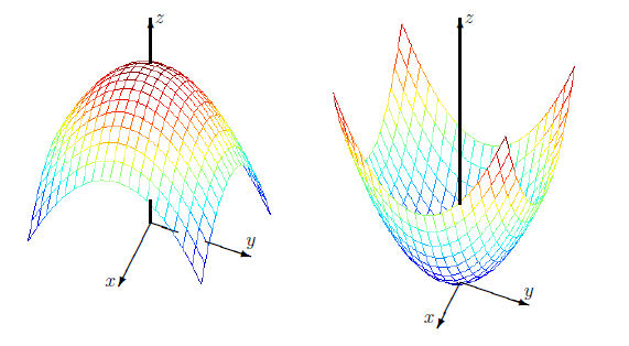
Graph of \(f(x)=1-x^2-y^2\) (left) and \(f(x)=x^2+y^2\) (right).

Theorem 8.5 If \(f\) has an extreme value at a point \({\bf x}_0\) which is an interior point of the domain of \(f\), then either

1. \(\nabla f({\bf x}_0)=0\),
2. or \(\nabla f({\bf x}_0)\) does not exist.

Proof: We show that if neither of 1 or 2 are true, then \({\bf x}_0\) cannot be an extreme point. So, assume that \(\nabla f({\bf x}_0)\neq 0\) (but it exists as a value). Hence \(f\) has (strictly) positive directional derivative in the direction of \(\nabla f({\bf x}_0)\). It follows that at \({\bf x}_0\) along the line with direction given by \(\nabla f({\bf x}_0)\) the function \(f\) is increasing and thus at \({\bf x}_0\) we can have neither a maximum or a minimum value. Hence, either \(\nabla f({\bf x}_0) = 0\) or it does not exist.

An example of a function with an extreme value at a point were the gradient does not exist is given in the next figure:

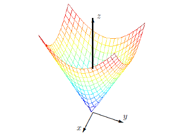
Graph of \(f(x)=\sqrt{x^2+y^2}\). The gradient is does not exist at the origin which is a point were the absolute minimum is attained.

Definition 8.4 An interior point \({\bf x}_0\) of the domain of \(f\) is named a

• stationary point if \(\nabla f({\bf x}_0)=0\);
• singular point if \(\nabla f({\bf x}_0)\) does not exist;
• critical point if it is a stationary or a singular point;
• saddle point if it is a critical point but not an extreme point.

The terminology saddle point comes from the typical shape of the graph of a function near a critical point that is not of extreme type; see the left picture in the figure below:

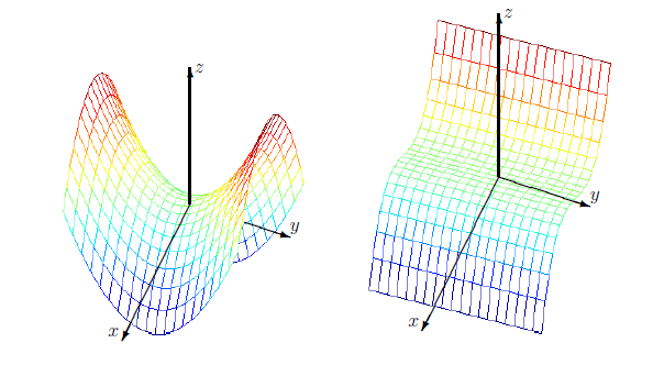
Examples of saddle points: graph of \(f(x)=-x^2+y^2\) (left) and \(f(x)=-x^3\) (right).

In conclusion, internal extreme points must be must be critical points. An extreme point, though, could also be located on the boundary of the domain. We can summarise our findings as follows.

Theorem 8.6 (Location of extreme points) Points where extreme values are attained are either critical (stationary or singular) points or boundary points.

Example 8.6 Find the global maximum and minimum value of the function \(f(x,y)=x^2+y^2\) on the unit disk \(D=\{(x,y)\in {\mathbb R}^2\,:\, x^2+y^2\le 1\}\).

A representation of the function \(f\) is given in the right caption of the figure above. Theorem 8.6 tells us that we can restrict our search to the collection of the critical and boundary points.

• Singular points: The function \(f\) does not have singular points.
• Stationary points: These are found by equating the gradient \(\nabla f(x,y)=(2x,2y)\) to zero, yielding the origin as the only stationary point. We have \(f(0,0)=0\).
• Boundary points: At the boundary \(x^2+y^2=1\) and thus \(f(x,y)=1\) (in this case, the boundary corresponds to a level curve).

As we knew already, the origin must be the point were the function has its global minimum equal to \(0\). The global maximum is attained at all points of the boundary of the domain \(D\) and is equal to \(1\).

Example 8.7 Find the hottest and coolest point of a triangular hot plate with vertices \(V_1=(0,-4)\), \(V_2=(6,-4)\), and \(V_3=(0,8)\) if its temperature is given by \(t(x,y)=x^2+xy+2y^2-3x+2y\).

It is understood that the domain occupied by the hot plate includes its boundary. Proposition 8.12 tells us that we can restrict our search for the maximum and minumum to the collection of the critical and boundary points.

• Singular points: The function \(t\) does not have singular points.

• Stationary points: These are found by equating the gradient \(\nabla t(x,y)=(2x+y-3,x+4y+2)\) to zero yielding the system of equations \[ \left\{ \begin{array}{l} 2x+y-3=0\\ x+4y+2=0 \end{array} \right. \qquad\Longleftrightarrow \qquad (x,y)=(2,-1). \]
  The point \(P=(2,-1)\) is the only stationary point of \(t\). It belongs to the region occupied by the hot plate and the temperature in it is \(t(2,-1)=4-2+2-6-2=-4\).

• Boundary points: The boundary is made of the three sides of the triangle. We study them one by one.
  • The side \(\overline{V_1V_2}=\{(x,-4)\,:\, x\in [0,6]\}\). The restriction of \(t\) on \(\overline{V_1V_2}\) is the function of one variable \(g(x)=x^2-7x+24\). This is a parabola concave up. Its minimum is achieved at the point such that \(g'(x)=2x-7=0\), that is \(x=7/2\). The maximum is achieved at both or either end point. We have \(f(0,-4)=g(0)=24\), \(f(7/2,-4)=g(7/2)=47/4=11.75\), and \(f(6,-4)=g(6)=18\).
  • On the side \(\overline{V_2V_3}=\{(x,-2x+8)\,:\, x\in [0,6]\}\) we get the function of one variable \(g(x)=7x^2-63x+144\). This is again a parabola concave up. Its minimum is achieved at the point such that \(g'(x)=14x-63=0\), that is \(x=63/14=9/2\). The maximum is achieved at both or either end point. We have \(f(0,8)=g(0)=144\), \(f(63/14,-1)=g(63/14)=2.25\), and \(f(6,-4)=g(6)=18\).
  • On the side \(\overline{V_1V_3}=\{(0,y)\,:\, y\in [-4,8]\}\) we get the function of one variable \(g(y)=2y^2+2y\). This is again a parabola concave up. Its minimum is achieved at the point such that \(g'(y)=4y+2=0\), that is \(y=-1/2\). The maximum is achieved at both or either end point. We have \(f(0,-4)=g(0)=24\), \(f(0,-1/2)=g(-1/2)=-1/2\), and \(f(0,8)=g(8)=144\).

By comparing all the values found, we conclude that the hottest point is the vertex \(V_3=(0,8)\) with \(t(0,8)=144\) and the coolest point is the internal point \((2,-1)\) with \(t(2,-1)=-4\).

8.5 Classification of stationary points of bivariate functions

Here we give a formal procedure of deciding if a stationary point is a maximum, a minimum or a saddle point. Recall the second derivative test for functions of one variable. Suppose that \(f=f(x)\) has a stationary point at \(x_0\), namely \(f'(x_0)=0\), and it has the second derivative there. Then, according to the second-derivative test,

• if \(f''(x_0)>0\), then \(f\) has a local minimum at \(x_0\);
• if \(f''(x_0)<0\), then \(f\) has a local maximum at \(x_0\);
• \(f''(x_0)=0\) the test gives no information (\(f\) can have a maximum, a minimum, or an inflection point).

For functions of several variables, the Hessian takes the role of the second derivative.

Definition 8.5 (Hessian) Let \(f\) be a function of \(2\) variables and \({\bf x}\) a point in the domain of \(f\). The Hessian matrix is defined as the matrix whose entries are all second partials of \(f\) at \({\bf x}\): \[ H_f({\bf x})=D^2f({\bf x}):=\left( \begin{array}{cc} f_{11}({\bf x}) & f_{12}({\bf x}) \\ f_{21}({\bf x}) & f_{22}({\bf x}) \end{array} \right). \]

As we have seen before the mixed partial derivatives are equal (if certain conditions are satisfied) so the Hessian matrix is symmetric.

Theorem 8.7 (Second derivative test) Suppose that \({\bf x}_0\) is a stationary point for \(f\) and that it is internal to the domain of \(f\). Further, assume that the Hessian is defined is symmetric at \(({\bf x}_0\))$.

• If the determinant of \(H_f({\bf x}_0)\) then:
  • if \(f_{11}({\bf x}_0)>0\), \(f\) has a local minimum at \({\bf x}_0\);
  • if \(f_{11}({\bf x}_0)<0\), \(f\) has a local maximum at \({\bf x}_0\);
• If the determinant of \(H_f({\bf x}_0)\) is negative, then \(f\) has a saddle point at \({\bf x}_0\);
• If the determinant of \(H_f({\bf x}_0)\) is zero then this test gives no information.

Example 8.8 Find and classify the stationary points of \(f(x,y)=x^4+x^2y^2-2x^2+2y^2-8\), \((x,y)\in {\mathbb R}^2\).

First of all, let us find the stationary points. These are found by solving the system \[ \left\{ \begin{array}{l} f_x(x,y)=4x^3+2xy^2-4x=2x(2x^2+y^2-2)=0\\ f_y(x,y)=2x^2y+4y=2y(x^2+2)=0 \end{array} \right. \Leftrightarrow \left\{ \begin{array}{l} x(2x^2-2)=0\\ y=0 \end{array} \right., \] whose solutions are the points \((0,0)\), \((1,0)\), and \((-1,0)\). To classify them, we calculate the hessian matrix: \[ H_f(x,y)= \left( \begin{array}{cc} 12x^2+2y^2-4 & 4xy\\ 4xy & 2x^2+4 \end{array} \right), \] and, in particular, \[ H_f(0,0)= \left( \begin{array}{cc} -4 & 0\\ 0 & 4 \end{array} \right),\qquad H_f(\pm 1,0)= \left( \begin{array}{cc} 8 & 0\\ 0 & 6 \end{array} \right). \] At \((0,0)\) the determinant is equal to \(-16<0\), hence \((0,0)\) is a saddle point. At \((\pm 1,0)\) the determinant is equal to \(48>0\) and \(A=8>0\) respecively, hence \((\pm 1,0)\) are both minimum points.

It is not always possible to solve the (nonlinear) equations yielding the stationary points. In these cases, a numerical procedure should be employed in order to find extreme values.

The steepest (or gradient) descent method is one such iterative procedure to approximate extreme values. It is based on the fact that the gradient gives the steepest descent. Suppose that we want to find the maximum of a function \(f\). Starting from any initial guess point \({\bf x}_0\), look for \({\bf x}_1\) along the direction of steepest descent \(\equiv\) the direction of the gradient at which \(f({\bf x}_1)> f({\bf x}_0)\), then iterate; see the picture below.

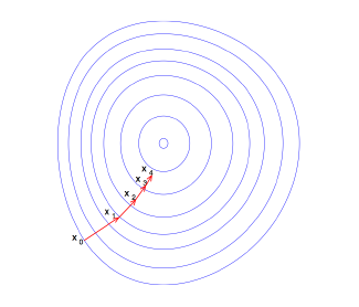
Few iterates of the gradient descent method. In blue the level curves of the target function.

Example 8.9 Verify that the cube has the most volume among all cuboids whose dimensions sum equals \(3a\).

We denote the dimensions of the solid by \(x,y,z\) so that the cuboid volume is \(V=xyz\) and the requirement on the edges length imposes the constraint \(x+y+z=3a\). Solving the latter equation with respect to \(z\) we have \(z=3a-(x+y)\) and substituting back in the volume formula yields \(V=V(x,y)=xy[3a-(x+y)]\), as a function of \(x,y\) whose domain must be the triangle \[ T=\{(x,y)\in {\mathbb R}^2: x,y> 0, x+y< 3a \}, \] so as to ensure that the volume is positive.

This function must have a maximum value inside the triangle and we know that at an extreme point the gradient must equal zero. The first partial are \[ V_x(x,y)=3ay-2xy-y^2,\qquad V_y(x,y)=3ax-2x^2-2xy, \] and setting both partial derivatives equal to zero we have \[ \left\{ \begin{array}{c} (3a-2x-y)y=0\\ (3a-x-2y)x=0. \end{array} \right. \] The only feasible solution is \(x=y=a\) which does belong to \(T\). Thus we get as expected \(x=y=z=a\). You may verify that the point obtained is indeed a maximum by applying the second derivative test.

Example 8.10 Find the distance between the point \((1,0,-2)\) and the plane \(x+2y+z=4\).

We know how to measure distances. The distance between any point \((x,y,z)\) and the point \(P=(1,0,-2)\) is \[ d=\sqrt{(x-1)^2+y^2+(z+2)^2}. \] Now, if the point \((x,y,z)\) is constrained on the plane, then \(z=4-x-2y\) and the distance becomes the function of two variables \[ d=d(x,y)=\sqrt{(x-1)^2+y^2+(6-x-2y)^2} \] This function must have a minimum and we may as well look for it by solving the equivalent problem: find \((x_0,y_0)\in {\mathbb R}^2\) such that \[ f(x,y)=(x-1)^2+y^2+(6-x-2y)^2, \] is minimised. As, \[ f_x(x,y)=4x+4y-14,\qquad f_y(x,y)=4x+10y-24, \] the stationary points of such function are found by solving the system of equations
\[ \left\{ \begin{array}{l} 2x+2y-7=0\\ 2x+5y-12=0. \end{array} \right. \] This is a linear system whose only solution is \((\frac{11}{6},\frac{5}{3})\). Thus the point in the plane that is closest to \(P\) is the point \((\frac{11}{6},\frac{5}{3},4-\frac{11}{6}-2\frac{5}{3})=(\frac{11}{6},\frac{5}{3},-\frac{7}{6})\) and the distance is \[ d=\sqrt{\left(\frac{11}{6}-1\right)^2+\left(\frac{5}{3}\right)^2+\left(-\frac{7}{6}+2\right)^2}=\sqrt{\left(\frac{5}{6}\right)^2+\left(\frac{5}{3}\right)^2+\left(\frac{5}{6}\right)^2}=\frac{5\sqrt{6}}{6}. \] You may verify that the point obtained is indeed a minimum by applying the second derivative test.

Example 8.11 We want to build a rectangular cardboard box with no top and of given volume \(V\) using the least quantity of cardboard. Find the length of the box’s edges by finding the minimum of the total surface function. Verify that the point you found is indeed a minimum applying the second derivatives test on such function.

We denote the dimensions of the solid by \(x,y,z\) so that the cuboid volume is \(V=xyz\). The task is to minimise the function \(S=xy+2yz+2xz\). Under the volume constraint \(z=V/(xy)\) and the surface function can be reduced to the function of two variables \[ S=S(x,y)=xy+\frac{2V}{x}+\frac{2V}{y},\qquad x,y>0. \] The minimum value must occur at a stationary point. Let us denote the stationary points \((x_0,y_0)\). The first partial derivatives are \[ S_x(x,y)=y-\frac{2V}{x^2},\qquad S_y(x,y)=x-\frac{2V}{y^2}. \] Setting these both to zero we have \[ \left\{ \begin{array}{l} x^2y=2V\\ xy^2=2V. \end{array} \right. \] Thus \(x^2y-xy^2=xy(x-y=0)\) yielding the only acceptable solution is \(x=y\) and \(x^3=2V\). Thus \(x_0=y_0=(2V)^{1/3}\) and then \(z_0=V/(x_0 y_0)=2^{-2/3}V^{1/3}=x_0/2\).

Let us verify by using the second derivatives test that the point found is indeed a minimum. We have \[ S_{xx}(x,y)=\frac{4V}{x^3},\qquad S_{yy}(x,y)=\frac{4V}{y^3},\qquad S_{xy}(x,y)=1, \] and, in particular, \[ S_{xx}(x_0,y_0)={4V \over x_0^3} = {4V \over 2V} = 2, \] and similarly \[ S_{yy}(x_0,y_0)=2,\qquad S_{xy}(x_0,y_0)=1. \] The determinant of the Hessian \[ S_{xx} (x_0,y_0)S_{yy}(x_0,y_0) - (S_{xy}(x_0,y_0))^2 \] is equal to \(3\) and thus is positive. Also \(S_{xx}(x_0,y_0)>0\), hence the given point is indeed a minimum.

In conclusion, the ideal box has a square base and height equal to half the base sides.

Example 8.12 Consider the function \(f(x,y)=\displaystyle\frac{xy}{1+x^2+y^2}\).

1. Find all stationary points of \(f\).
2. Classify all stationary points of f as maximum, minimum, or saddle point. Justify your arguments.
3. Find the absolute maximum and minimum values of the function \(f\) on the unit disk centred in the origin. List all points \((x,y)\) at which the extreme values are attained.

The stationary point are those points at which the gradient is zero. We have: \[ f_x(x,y)=\frac{y+y^3-x^2y}{(1+x^2+y^2)^2},\qquad f_y(x,y)=\frac{x+x^3-xy^2}{(1+x^2+y^2)^2}, \] and we are looking for the points at which the partial derivatives are simultaneously zero: \[ \left\{ \begin{array}{l} y(y^2-x^2+1)=0,\\ x(x^2-y^2+1)=0, \end{array} \right. \quad\Leftrightarrow\quad \left\{ \begin{array}{l} y=0\quad \text{or}\quad y^2-x^2+1=0,\\ {\rm and}\\ x=0\quad \text{or}\quad x^2-y^2+1=0, \end{array} \right. \] This system of equation has the only real solution \((x,y)=(0,0)\), so the origin is the only stationary point.

The second derivative test does not yield any information as the Hessian at the origin is zero. The origin is a saddle point, as it is obvious from a direct inspection. Indeed, \(f(0,0)=0\) and \(f\) takes both positive and negative values in any neighbourhood of the origin (\(f(x,y)>0\) if \(xy>0\), that is in the first and third quadrant, and \(f(x,y)<0\) if \(xy<0\), that is in the second and forth quadrant), so it cannot be neither a maximum or a minimum. Another way to see this is to inspect \(f\) along a couple of well-chosen lines: for instance, when restricted on the line \(y=x\) the function \(f\) has a minimum at \(x=0\), while when restricted on the line \(y=-x\) it has a maximum there.

The function \(f\) must have global maximum and minimum on the bounded and closed region \(\{x^2+y^2\le 1\}\). As the function \(f\) is regular and does not have any stationary point that are either a maximum or a minimum, the maximum and minimum values must be taken on the boundary, which is given by \(x^2+y^2= 1\). Here we have \[ f(x,\pm \sqrt{1-x^2})=\pm \frac{x\sqrt{1-x^2}}{2},\qquad x\in[-1,1]. \tag{8.2} \] We start by studying the function \[ g(x)=f(x,\sqrt{1-x^2})=\frac{x\sqrt{1-x^2}}{2},\qquad x\in[-1,1], \] whose derivative is given by \[ g'(x)=\frac{1-2x^2}{2\sqrt{1-x^2}},\qquad\forall x\in (-1,1). \] Its stationary points are given by the solutions of the equation \(g'(x)=0\) which are \(x=\pm \frac{\sqrt{2}}{2}\). Clearly, by considering the minus sign in (8.2), we would obtain the same result. Thus the global maximum and minimum must be taken at one or more of the points \[ \left (\pm\frac{\sqrt{2}}{2},\frac{\sqrt{2}}{2} \right ), \quad \left (\frac{\sqrt{2}}{2},\pm\frac{\sqrt{2}}{2} \right ). \] Then \[ f \left (\pm\frac{\sqrt{2}}{2},\pm\frac{\sqrt{2}}{2} \right )= \frac{1}{4},\qquad f \left (\pm\frac{\sqrt{2}}{2},\mp\frac{\sqrt{2}}{2} \right )=- \frac{1}{4}, \] hence, on the unit circle, the global maximum of \(f\) is \(1/4\), taken at \(\left (\pm\frac{\sqrt{2}}{2},\pm\frac{\sqrt{2}}{2} \right )\) and the global minimum is \(-1/4\) taken at \(\left (\pm\frac{\sqrt{2}}{2},\mp\frac{\sqrt{2}}{2} \right )\).

As before, we should consider the end points of the intervals i.e. \((\pm 1, 0)\), but \(f(\pm 1, 0)=0\) so are not extreme values.

8.5.1 Test yourself

8.6 Challenge yourself

1. Let \(f(x,y,z)=0\). By considering a curve \({\bf r}(t)\) lying in the surface Show that \(\nabla f\) is perpendicular to the the surface. You should use the fact that {}’(t)$ is tangential to the surface.
2. Investigate Lagrange multipliers. These are used for contrainted optimisation. See if they make the algebra in solving the hot plate problem in Example 8.7 more straightforward.