Chapter 2 Integration

Integration is the term we use to describe adding together an infinite number of infinitesimally small bits of something to make up the whole. For instance, in order to work out the length of a curve, we might break it into a lot of straight lines, and then add the lengths of these lines together:

In the next bit of code we estimate the length of a semi circle of radius 1. What answer should we expect?

semicirc <-function(t){
  (1-t^2)^(1/2)
  }

npts <- 8 # as.integer(readline(prompt="Number of points:"))

div<-2/npts

x=seq(-1,1, by=div)

y=x[0:npts+1]

  plot(y,semicirc(y),main="f(x)=sqr(1-x^2)",
ylab="f(x)",
type="l",
col="blue")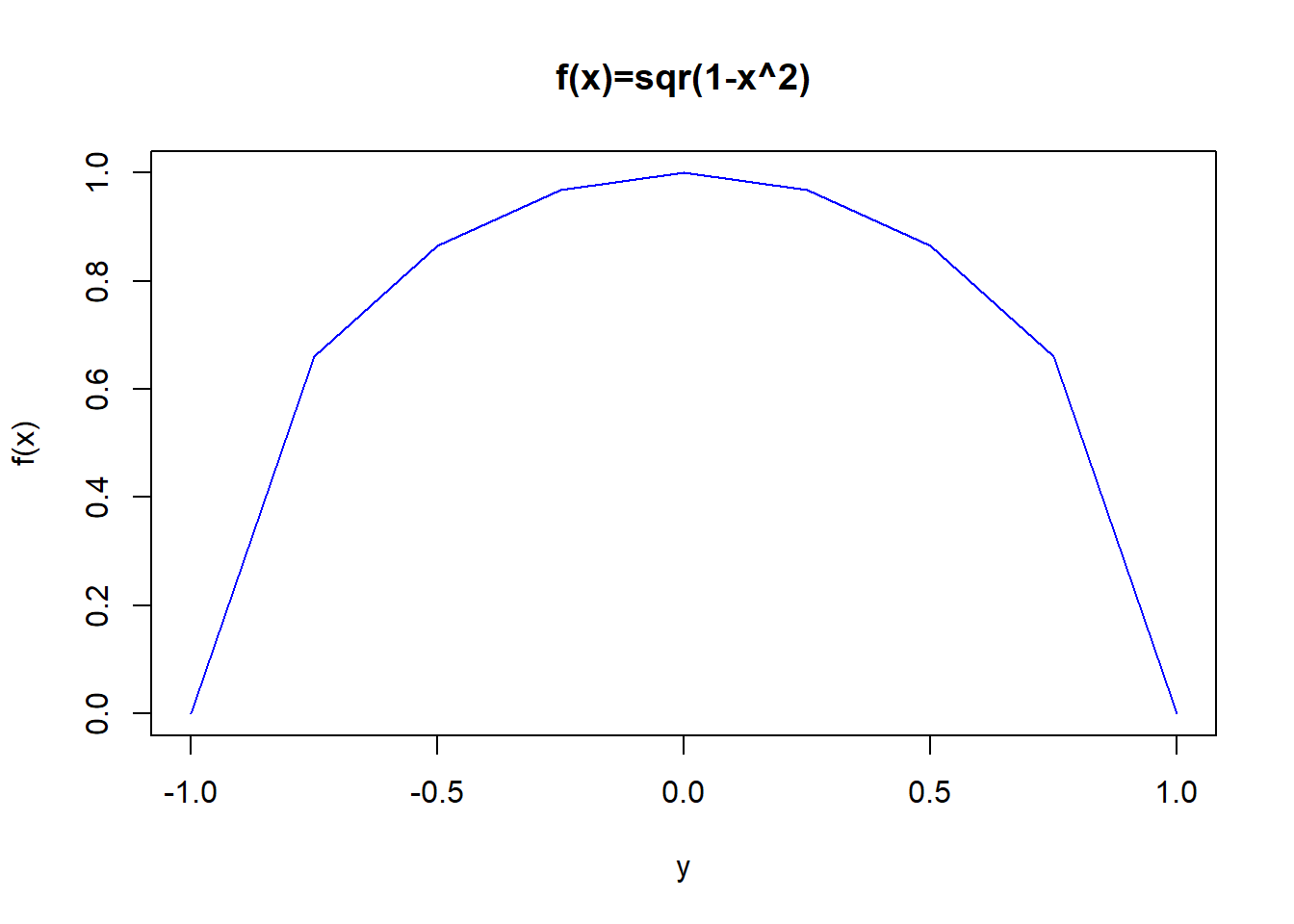

  lentot<-0
  for (i in 1:npts){
    lentot<-lentot+((y[i+1]-y[i])^2+(semicirc(y[i+1])-semicirc(y[i]))^2)^(1/2)
  }
  
  print(lentot)

## [1] 3.104496

2.1 Integration of Polynomials

In this section we will look at the integration of polynomials by approximating the area under the curve by rectangles. Now let us think about the function \(y=1\) on the interval \([0,t]\), for some \(t>0\).

Then the area of the rectangle is \(t\) and we say the integral of \(y=1\) between \(0\) and \(t\) is \(t\), and we write \[ \int_0^t 1 dx = t. \]

Now let us consider the function \(y=x\) on the interval \([0,t]\), for some \(t>0\). Here is a picture.

It is clear that the area of this is the area of an isosceles right-angled triangle of side length \(t\) which is \(t^2/2\). Hence, the integral of \(y=x\) between \(0\) and \(t\) is \(t^2/2\). We write this \[ \int_0^t x dx = {t^2 \over 2}. \]

Unfortunately, integrating other functions is not so straightforward. The next bit of code shows how to compute an esimate to the area under \(y=x^2\) using rectangles.

parab <-function(x){
  
  x^2
  
}

npts <- 16 # as.integer(readline(prompt="Number of points:"))

div<-1/npts

x <- seq(0,1,0.01)
  plot(x,parab(x),main="f(x)=x^2",
ylab="f(x)",
type="l",
col="blue")
  
  
  area<-0
  for (i in 1:npts){
    area<-area+(i-1)^2/npts^3
    rect((i-1)/npts,0,i/npts,(i-1)^2/npts^2,col="red")
  }

  print(area)

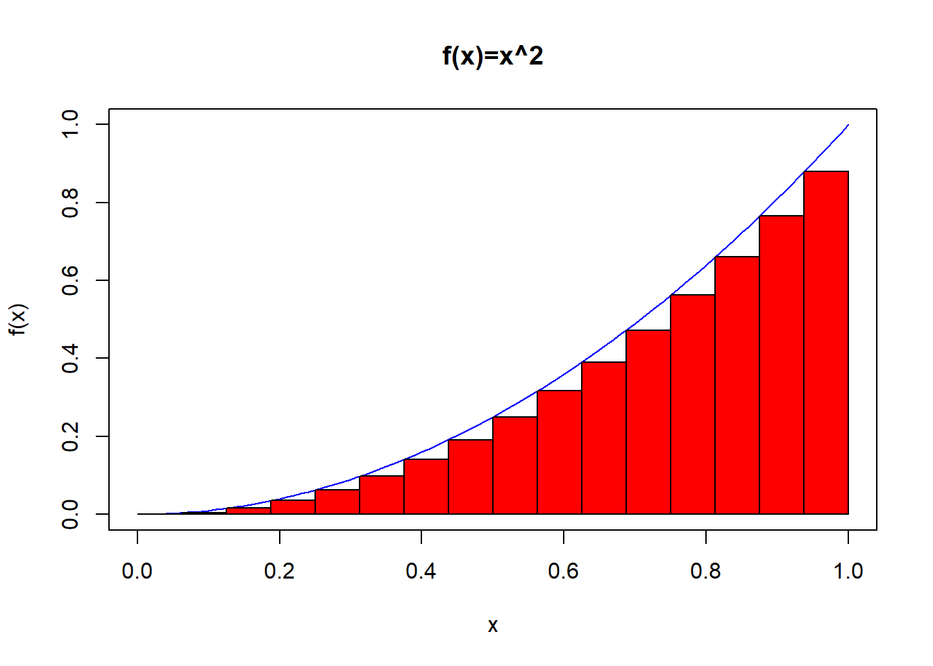
## [1] 0.3027344

Theorem 2.1 The integral of \(y=x^2\) between 0 and \(t\) is \(t^3/3\).

Proof: Let us divide the interval \([0,t]\) into \(n\) equal parts, each of width \(t/n\). Let us write \(x_i=it/n\), \(i=0,1,\cdots,n\). Then the height of the \(i\)th rectangle is \(x_{i-1}^2\) (the left hand end of the first rectangle is \(x_0=0\)). If we substitute \(x_{i-1}=(i-1)t/n\), we get the height \((i-1)^2t^2/n^2\). Hence the area of the \(i\)th rectangle is \[ R_i = {t \over n}{(i-1)t^2 \over n^2}={t^3 \over n^3} (i-1)^2. \] Thus the total area of the rectangles is \[ A_n = \sum_{i=1}^n R_i = {t^3 \over n^3} \sum_{i=1}^n (i-1)^2 = {t^3 \over n^3} \sum_{i=1}^{n-1} i^2. \tag{2.1} \]

For the moment we will just use the known fact that \[ \sum_{i=1}^m i^2 = {1 \over 6} m(m+1)(2m+1) \] to see that \[ \sum_{i=1}^{n-1} i^2 = {1 \over 6} (n-1)n(2n-1)={1 \over 3}n^3-{1 \over 2}n+{1 \over 6}n. \]

Substituting the last equation intp we get \[ A_n = {t^3 \over n^3} \left ( {1 \over 3}n^3-{1 \over 2}n+{1 \over 6}n \right ) = {t^3 \over 3} - {1 \over 2} {t^3 \over n} + { 1 \over 6}{t^3 \over n^2}. \] Now, as \(n \rightarrow \infty\) the second and third terms tend to zero (we will make these terms more precise later in the course), leaving us with the area \[ A = \lim_{n \rightarrow \infty} A_n = {t^3 \over 3}. \Box \]

Remark. What do you notice about the approximations for the area? Suppose you used rectangles with height given by the value of the function at the left hand end of the interval? Copy and paste the code for integrating into a new code cell. Change the programme so that the height of the rectangle is the value of the function in the middle of the cell. Recompute the estimates to the area. What do you notice. Can you explain this.

Remark. Let the number \(a_n\), \(n=0,1,2,\cdots\) be the estimate to the integral of \(x^2\) from above with \(2^n\) rectangles. Then (to 5 decimal places we have) \[\begin{eqnarray} a_0 & = & 0.12500 \\ a_1 & = & 0.21875 \\ a_2 & = & 0.27344 \\ a_3 & = & 0.30273 \\ a_4 & = & 0.31787 \\ a_5 & = & 0.32556 \\ a_6 & = & 0.32944 \\ a_7 & = & 0.33138 \\ a_8 & = & 0.33235 \\ a_9 & = & 0.33284. \end{eqnarray}\] This is an example of a Cauchy sequence, which is a fancy name for a sequence where the differences between numbers in the sequence get closer and closer as you go along the sequence. \[\begin{eqnarray} |a_0-a_1| & = & 0.09375 \\ |a_1-a_2| & = & 0.05469 \\ |a_2-a_3| & = & 0.02930 \\ |a_3-a_4| & = & 0.01514 \\ |a_4-a_5| & = & 0.00769 \\ |a_5-a_6| & = & 0.00388 \\ |a_6-a_7| & = & 0.00194 \\ |a_7-a_8| & = & 0.00095 \\ |a_8-a_9| & = & 0.00049. \\ \end{eqnarray}\] In numerical calculations we often get sequences like this. The question (which we will return to) is do such sequences converge to a number? This forms a central question for this module. You will also notice that the sequence increases but never gets bigger than 0.5 say. We say that the sequence is monotone increasing and that it is bounded above. We will want to talk about such sequences too.

2.1.1 The cultural heritage of mathematics

Hasan Ibn al-Haytham discovered the sum formula for the fourth power, using a method that could be generally used to determine the sum for any integral power. He used this to find the volume of a paraboloid. He could find the integral formula for any polynomial without having developed a general formula.

2.1.2 Test Yourself

Now you can test your understanding of integration with the following question. Put your answers in to 2 decimal places.

2.2 Challenge yourself

Show that \[ \int_0^t x^3 dx = {t^4 \over 4}. \]
Use Q2 from Section 1.5 to show that for any \(m \in {\mathbb N}\) \[ \int_0^t x^m dx = {t^{m+1} \over m+1}. \]
Let \(L_n\) be the rectangle rule estimate to \[ I=\int_0^1 x^2 dx \] using the left hand end rectangles. Let \(R_n\) be the estimate using the right hand rectangles. Show that there is a positive constant \(C\) such that \[ \left |I-{L_n+R_n \over 2} \right | \le {C \over n^2}. \] Explain why \((L_n+R_n)/2\) is a better estimate than either \(L_n\) or \(R_n\).
Let \(M_n\) be the estimate \(I\) above using the height of the rectange at the middle of the interval as opposed to the left or right end. Show that there is a positive constant \(D\) \[ |I-M_n| \le {D \over n^2}. \] Explain why \(M_n\) is a better estimate than \(L_n\) or \(R_n\). Is it a better esimtate than \((L_n+R_n)/2\)?