Chapter 5 Taylor Series

One of the most useful tools for solving problems in mathematics is the capability to approximate an arbitrary function using polynomials. There are a number of different methods for approximating functions that you will find out about in your degree including - Taylor series - Fourier series - Interpolation - wavelets (maybe) - radial basis functions (Jeremy’s research area) - neural networks (Alexander Gorban’s and Ivan Tyukin’s research areas).

5.1 Taylor polynomials

We use polynomials because they can be computed on a machine only using multiplication and addition.

Definition 5.1 A polynomial is a function of the form $$p_n(x) = \sum_{i=0}^n a_i x^i,$$ for some $n \in {\mathbb N}$. We call this a monomial, if there is only one term in this expansion. The number $n$ is called the degree of the polynomial (we assume that $a_n \neq 0$).

We have already met one Taylor polynomial, in Section 3.2 when we were looking at approximating a function by its tangent in Newton’s method. The idea for Taylor series is that we will match the each derivative of a polynomial with the derivative of the function at a particular point $b$ (this is called Hermite interpolation’’ in the trade).

We are going to start with the simple case $b=0$. Let us try with a degree 2 polynomial and an arbitrary function $f$. Let $$p_2(x) = a_0+a_1 x +a_2 x^2, \tag{5.1}$$ and we want $$\begin{eqnarray} p_2(0) & = & f(0), \\ p_2^{'}(0) & = & f^{'}(0), \\ {\rm and} \; p_2^{''}(0) & = & f^{''}(0). \\ \end{eqnarray}$$ If we let $x=0$ in (5.1) we get $$a_0 = f(0).$$ Let us now differentiate $p_2^{'}(x)=a_1+2a_2 x$. If we substitute $x=0$ we get $$p_2^{'}(0)=a_1=f^{'}(0).$$ Differentiating a second time we get $p_2^{''}(x)=2a_2$. Substituting in $x=0$ gives $$p_2^{''}(0)=2a_2=f^{''}(0),$$ so that $$a_2 = {f^{''}(0) \over 2}.$$ Therefore our approximating polynomial is $$p_2(x)=f(0)+f^{'}(0) x+{f^{''}(0) \over 2}x^2. \tag{5.2}$$

Example 5.1 Let us test the idea out on a particular function $f(x)=\sqrt{1+x}$. Then $$\begin{eqnarray} f(0) & = & \sqrt{1} = 1 \\ f'(x) & = & {1 \over 2 \sqrt{1+x}} \Rightarrow f'(0)={1 \over 2} \\ f''(x) & = & -{1 \over 4 (\sqrt{1+x})^3} \Rightarrow f''(0) = -{1 \over 4}. \end{eqnarray}$$ Substituting into (5.2) we get $$P_2(x)=1+{x \over 2} - {x^2 \over 8}x^2.$$

Now let us see if this is a good approximation. Let us use the last equation to approximate $\sqrt{1.1}=1.0488088$ to 7 decimal places. Our approximation is $$P_2(0.1) = 1+{0.1 \over 2} - {(0.1)^2 \over 8} = 1.04875.$$ Hence our estimate is out by approximately $0.00005$.

Suppose we use $p_2$ to approximate $\sqrt{1.2}=1.0954451$ to 7 decimal places. Our approximation is $$P_2(0.2) = 1+{0.2 \over 2} - {(0.2)^2 \over 8} = 1.095.$$ Hence our estimate is out by approximately $0.0004$, so the error has increased almost 10 times. We will return to theoretical error estimates for Taylor series next semester.

We can see above that the higher the degree of the polynomial approximation, the better it gets. In this link

(http://mathfaculty.fullerton.edu/mathews/a2001/Animations/Interpolation/Series/Series.html)

you can examples of Taylor series approximations for a variety of functions and observe how they improve as you increase the degree of the polynomial.

More generally, we can look at the Taylor series for a point $b$. In order to compute this it is more convenient to use a different basis for the polynomials. A basis is an idea that you will see more of in linear algebra. It is a set of objects which we use to represent our information. For the point $b$ I would like my polynomial to be written in the form $$p_n(x)=a_0+a_1(x-b)+a_2(x-b)^2+\cdots+a_n(x-b)^n = \sum_{i=0}^n a_i(x-b)^i.$$ It will become clear in a second why this is a good idea. We will find $a_i$ by matching the $i$th derivative of $p_n$ with the $i$th derivative of our target function $f$, which we are trying to approximate. If we differentiate $p_n$ $j$ times we get $$p_n^{(j)}(x) = j! a_j+(j+1)!a_{j+1}(x-b)+{(j+2)! \over 2}(x-b)^2+\cdots+a_n{n! \over (n-j)!}(x-b)^{n-j}.$$ If we put $x=b$ in this we see that $$p_n^{(j)}(b) = j! a_j.$$ Since we wish to make $p_n^{(j)}(b)=f^{(j)}(b)$, we obtain $$a_j = {f^{(j)}(b) \over j!}.$$ If we had used $$p_n (x)=a_0+a_1x+a_2x^2+\cdots+a_nx^n,$$ then all of the terms greater than the $j$th term would not have become 0 and we would have got a horrible mess. Thus we have the following definition for the Taylor polynomial:

Definition 5.2 (Taylor polynomial) Let $f$ have $n$ continuous derivatives at $b$. Then the Taylor polynomial for $f$ at $b$ is $$\sum_{j=0}^n {f^{(j)}(b) \over j!} (x-b)^j$$

In the next code we plot degree 0, 1, 2, and 3 Taylor polynomials.

        fun <- function(x){
            sin(x) # The function we are approximating
        }

        dfun <-function(x){
            cos(x) # the derivative of the function
        }

        d2fun <- function(x){

            -sin(x) # second derivative
        }

        d3fun <- function(x){

            -cos(x) # third derivative
        }

        line <- function(x,b,fb,dfb){ # This is the equation of a line of gradient dfb through (b,fb)

            fb+dfb*(x-b)

        }

        quad <-function(x,b,fb,dfb,d2fb){ # inputs are the derivatives at the point b

            fb+(x-b)*dfb+(x-b)^2/2*d2fb # degree 2 Taylor polynomial

        }

        cubic <-function(x,b,fb,dfb,d2fb,d3fb){ # inputs are the derivatives at the point b

            fb+(x-b)*dfb+(x-b)^2/2*d2fb+(x-b)^3/6*d3fb # degree 2 Taylor polynomial

        }

        b <- pi/6 # the point at which we compute the tangent

        # Plot the function and the tangent on an interval around the point

        x <- seq(b-2,b+2,0.01)
        plot(x,line(x,b,fun(b),dfun(b)),main="Degree 1, 2 and 3 Taylor poynomials",
             ylab="f(x)",
             type="l",
             col="blue")
        lines(x,fun(x),col="green")
        lines(x,quad(x,b,fun(b),dfun(b),d2fun(b)),col="red")
        lines(x,cubic(x,b,fun(b),dfun(b),d2fun(b),d3fun(b)),col="black")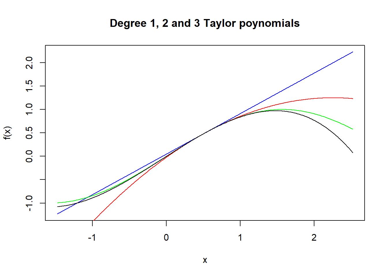

Definition 5.3 (Taylor series) Let $f$ have infinite continuous derivatives at $b$. Then the Taylor series for $f$ at $b$ is $$\sum_{j=0}^\infty {f^{(j)}(b) \over i!} (x-b)^j$$

Remark. The selection of a good basis is one of the most important mathematical skills to develop. A bad choice of basis can make the problem almost impossible to solve. A good choice can make it trivial.

Example 5.2 The Taylor series for $\cos x$ and $\sin x$ at $b=0$ are $$\cos x = \sum_{j=0}^\infty {(-1)^j \over (2j)!} x^{2j},$$ $$\sin x = \sum_{j=0}^\infty {(-1)^{2j+1} \over (2j+1)!} x^{2j+1}.$$

Example 5.3 Compute the Taylor series for $f(x)={1 \over 1+x}$ at $x=1$. How many terms in the series do you need to get 2 decimal places of accuracy for estimating $f(1.1)$?

The formula for the Taylor series at $x=1$ is $$f(x)=\sum_{j=0}^\infty {f^{(j)}(1) \over j!} (x-1)^j.$$ The $j$th derivative of $f$ in this case (it is easy to check) $$f^{(j)}(x) = (-1)^j {j! \over (1+x)^{j+1}}.$$ Hence $$f^{(j)}(1) = (-1)^j {j! \over 2^{j+1}}.$$ Substituting this into the formula for the Taylor series we have $$f(x)=\sum_{j=0}^\infty {(-1)^j \over 2^{j+1}} (x-1)^j.$$ Thus $$f(1.1)=\sum_{j=0}^\infty {(-1)^j \over 2^{j+1}} (0.1)^j.$$ In order to approximate the value at $x=1.1$ to 2 decimal places we look for the first term in the expansion which is less than 0.005, as this will not change the calculation to 2 d.p. When $j=2$ the term in the expansion is $${(-1)^2 \over 2^{3}} (0.1)^2 = 1/800.$$ This is less than 0.005 in size. Thus we need only two terms: $$f(1.1) \approx {1 \over 2} - {1\over 40} = 0.475.$$ The actual value is $10/21=0.476190476190476$ and so we have two decimal places.

5.1.1 Test yourself

5.1.1.1 Functions of the form $f(x)=(A+Bx)^{m/n}$.

5.1.1.2 Functions of the form $y=A\exp(mx)$.

5.2 Polar form for complex numbers

Richard Feynman, the famous physicist called the following equation ‘’our jewel’’ and ‘’the most remarkable formula in mathematics’’.

Richard Feynmann

Theorem 5.1 (Polar coordinates for complex numbers) For any real number $\theta$ $$\exp(i \theta) = \cos \theta + i \sin \theta.$$

Using the Taylor series for $\exp(i \theta)$ we have $$\begin{eqnarray*} \exp(i \theta) & = & \sum_{n=0}^\infty {(i \theta)^n \over n!}\\ & = & \sum_{n=0}^\infty {i^n \theta^n \over n!}. \end{eqnarray*}$$ Now, $i^2=-1$, $i^3=-i$ and $i^4=1$, so that $$\begin{eqnarray*} \exp(i \theta) & = & \sum_{n=0}^\infty {i^n \theta^n \over n!} \\ & = & 1+i \theta - {\theta^2 \over 2!} - i{\theta^3 \over 3!}+{\theta^4 \over 4!}+{\theta^5 \over 5!}- \cdots \\ & = & 1 - {\theta^2 \over 2!}+{\theta^4 \over 4!}+ \cdots + i (\theta - {\theta^3 \over 3!} + {\theta^5 \over 5!} + \cdots) \\ & = & \left (\sum_{n=0}^\infty {(-1)^n \over (2n)!} \theta^{2n} \right )+i\left ( \sum_{n=0}^\infty {(-1)^{2n+1} \over (2n+1)!} \theta^{2n+1} \right ) \\ & = & \cos \theta + i \sin \theta.\qquad \Box \end{eqnarray*}$$

Thus $\exp(i \theta)$ is a complex number with real part $\cos \theta$ and imaginary part $\sin \theta$. If plot this we can see that $\exp(\theta \theta)$ is a complex number of length 1 at angle $\theta$ to the real axis.

Polar coordinates

Definition 5.4 (Polar form of complex number) Any complex number can be written in polar form $$z=x+iy=r\exp(i \theta),$$ where $r=\sqrt{x^2+y^2}$ is called the of the complex number (written $|z|$, and $\theta=\arctan(y/x)$ is called the argument of the z, written ${\rm arg \,} z$.

Example 5.4 Write $z=2+4i$ in the form $z=r\exp(i \theta)$.

The modulus of $z$ $r=\sqrt{2^2+4^2}=\sqrt{20}$. We have $\theta={\rm arg \,} z=\arctan(4/2)=1.11$ radians.

In this code you can change the real and imaginary parts of the input complex number and see what the modulus and argument are. The code is written so that $-\pi<\theta \le \pi$.

x <- -2
y <- -3

r <- (x^2+y^2)^(1/2)
theta=atan(y/x)
if (x<0) { # if x is negative we will have computed the wrong anlge and need to add pi.
  theta<-theta+pi
}

if (theta>=pi) { # Put theta in the range -pi to pi
  theta<-theta-2*pi
}

cat('Modulus = ',r,'   Argument = ',theta)

## Modulus =  3.60555127546    Argument =  -2.15879893034

5.2.1 Test yourself

Test your knowledge of polar and cartesian forms of complex numbers.

5.3 Challenge yourself

1. Use Taylor’s theorem to prove the Binomial expansion $$(1+x)^\alpha = 1 + \alpha x + {\alpha(\alpha-1) \over 2} x^2 + \cdots.$$ Test this formula out for $\alpha=1/2$, $x=0,1/2,1,-1/2,-1$. Is there any place that the formula does not work. Can you explain this.
2. Can you use the Taylor series for $\exp(x)$ and the fact that $\log x$ is the inverse function for $\exp(x)$ to compute the Taylor series for $\log(1+x)$? This question is exploratory.
3. Use Euler’s formula $\exp(i \theta)=\cos \theta+i \sin \theta$ to show the two formulae $$\begin{eqnarray*} \cos(\theta+\phi) & = & \cos \theta \cos \phi - \sin \theta \sin \phi \\ \sin(\theta+\phi) & = & \sin \theta \cos \phi + \cos \theta \sin \phi. \end{eqnarray*}$$ Try to prove these formulae another way.
4. How many cube roots of 1 are there if we allow complex numbers. Plot these roots on the complex plane. What shape do these roots make? How about fourth roots and fifth roots?