Chapter 7 Functions of two or more variables

7.1 Introduction

‘’If I have seen farther than other men, it is because I have stood on the shoulders of giants.’’

Isaac Newton (1642-1727)

‘’If I have not seen as far as others, it is because giants were standing on my shoulders.’’

Hal Abelson (1947-)

In this chapter we are going to study real functions of two variables, that is, functions $f:{\mathbb R} \times {\mathbb R} \rightarrow {\mathbb R}$ associating to each pair of real number $(x,y)$ a real number $y=f(x,y)$. Next semester we will look at the concepts of limit and continuity. In this chapter we will look at derivatives, for the purpose of understanding gradient on surfaces, as well as finding maxima and minima in two dimensions.

We begin with some examples.

Example 7.1 The simplest example of a surface is a plane, which is a linear function: $$z=ax+by+c, \quad a,b,c \in {\mathbf R}.$$ In the example below $z=3x+4y+5/2$.

Example 7.2 Suppose we want to describe the elevation above see level of each point on the surface of a mountain. For simplicity, suppose that the mountain just looks like a cone, with the base at sea level. The altitude can be represented by the function $$\begin{eqnarray*} f:D & \longrightarrow & {\mathbb R} \\ z & = & f(x,y), \end{eqnarray*}$$ associating to each point in the cone’s base to the corresponding altitude. Here, the cone base is represented by a subset of the real plane $D\subset{\mathbb R}^2$: this is the map of the mountain. Each point in $D$ can be uniquely represented by a pair of coordinates $(x,y)$. An appropriate function here is $$z=2-\sqrt{x^2+y^2},$$ and the region $D=\{(x,y): x,y \in [-1,1] \}$.

Example 7.3 To represent the temperature in each point of your study room, we can use a function of three variables: $$f:D \longrightarrow {\mathbb R}, \qquad T=f(x,y,z).$$ Here, the domain $D\subset{\mathbb R}^3$ describes the room and the the output value $T$ the temperature as a function of position in space. For instance $$T=(a^2-x^2)(y^2-b^2)(z^2-c^2),$$ where $D=[-a,a] \times [-b,b] \times [-c,c]$. Obvioulsy it is difficult to visualise such functions, and it is a skill to find a good way to visualise information.

Example 7.4 What if we want also to keep track on how the temperature changes with time? Well, just add one more variable, $t$ for time, and describe the temperature as a function of both position in space and time: $$f:D\longrightarrow{\mathbb R}, \qquad T=f(t,x,y,z).$$ Here, the domain $D\subset {\mathbb R}^4$ describes the time-space domain given by the room the time interval of interest. For instance, suppose the temperature decays in time exponentially then we might have a formula of the type $$T=(a^2-x^2)(y^2-b^2)(z^c-c^2)\exp(-2t),$$ with $D=[0,\infty) \times [-a,a] \times [-b,b] \times [-c,c]$.

7.2 Partial Derivatives

If we imagine ourselves on a mountainside, we know that the slope can be different in different directions. This is how we skiers manage to get down very steep slopes slowly, by moving across the slope. We can work out how much things are changing along a particular line. In the following picture from Mathsinsight.org https://mathinsight.org/

We are looking at the changes to the function $f(x,y)$ if we fix $y=b$. For instance, suppose we think about the cone $f(x,y)=2-\sqrt{x^2+y^2}$, and put $y=-0.5$, then we are looking at the function $g(x)=f(x,0.5)=2-\sqrt{x^2+1/4}$. Then we can explore the rate of change of $f$ along the line $y=-0.5$ by differentiating $g$ with respect to $x$.

Definition 7.1 (Partial derivatives of a function of two variables) Let $f$ be a function of two variables $x,y$. The partial derivatives of $f$ with respect to $x$ and $y$ are, respectively, $$\begin{eqnarray*} f_x(x,y) & = & \lim_{h\rightarrow 0}\frac{f(x+h,y)-f(x,y)}{h},\\ f_y(x,y) & = & \lim_{h\rightarrow 0}\frac{f(x,y+h)-f(x,y)}{h}. \end{eqnarray*}$$ The partial derivatives measures the rate of change of $f$ with respect to one variable.

Remark. The following are other notations for first partial derivatives you should be aware of: $$\begin{eqnarray*} f_x(x,y)=f_1(x,y)& = & \frac{\partial f}{\partial x}(x,y)=D_1 f(x,y),\\ f_y(x,y)=f_2(x,y) & = & \frac{\partial f}{\partial y}(x,y)=D_2 f(x,y). \end{eqnarray*}$$

Finding the partial derivatives of a function, is pretty straightforward if you know how to take derivatives of single-variable functions. Indeed, by definition, the partial derivative, say, with respect to $x$, is the derivative of the function when $y$ is fixed. The procedure is illustrated with the following examples.

Example 7.5 Let $f(x,y)=x^2y^3+3x^2y$. Then $$\begin{eqnarray*} f_x(x,y)& = & 2xy^3+6xy,\\ f_y(x,y)& = & 3xy^2+3x^2. \end{eqnarray*}$$

The following is a more complicated example.

Example 7.6 Find the first partial derivatives of the function $f(x,y)=x \arctan (xy)+\exp(2y)$. Evaluate the partial derivatives at the point $(x,y)=(1,0)$.

Thinking of $y$ as a consant we have $${\partial f \over \partial x} = \arctan (xy) + {xy \over 1+(xy)^2}=0,$$ when $(x,y)=(1,0)$. With $x$ as a constant we have $${\partial f \over \partial y} = {x^2 \over 1+(xy)^2}+2\exp(2y)=3.$$ when $(x,y)=(1,0)$.

Here is a video with some more examples:

YOutube clip with more examples

7.2.1 Test yourself

7.3 Partial derivatives of higher order

Again, we consider first just functions of two variables. Suppose that $f$ is a function of the two variables $x,y$ admitting first partial derivatives in its domain of definition. As the partial derivatives $f_x$ and $f_y$ are again functions of $x$ and $y$, they may themselves possess partial derivatives $(f_x)_x$, $(f_x)_y$, $(f_y)_x$ $(f_y)_y$. These functions are the second-order partial derivatives of $f$. For these, we introduce the following notation. The two pure second partial derivatives $$\begin{eqnarray*} f_{xx}& = & f_{11}=\frac{\partial^2 f}{\partial x^2}=\frac{\partial }{\partial x}\left(\frac{\partial f}{\partial x}\right):=(f_x)_x,\\ f_{yy} & = & f_{22}=\frac{\partial^2 f}{\partial y^2}=\frac{\partial }{\partial y}\left(\frac{\partial f}{\partial y}\right):=(f_y)_y, \end{eqnarray*}$$ and two mixed second partial derivatives $$\begin{eqnarray*} f_{xy} & = & f_{12}=\frac{\partial^2 f}{\partial y\partial x}=\frac{\partial }{\partial y}\left(\frac{\partial f}{\partial x}\right):=(f_x)_y,\\ f_{yx} & = & f_{21}=\frac{\partial^2 f}{\partial x\partial y}=\frac{\partial }{\partial x}\left(\frac{\partial f}{\partial y}\right):=(f_y)_x. \end{eqnarray*}$$ These are, by definition, calculated by taking partial derivatives of already calculated partial derivatives.

Example 7.7 Calculate the second partial derivative of the function $f(x,y)=y\exp(x^2)+xy$.

We start by calculating the first partial derivatives: $$f_x(x,y)=2xy\exp(x^2)+y,\qquad f_y(x,y)=\exp(x^2)+x,$$ and then get the second partial derivatives by taking the partial derivatives of $f_x$ and $f_y$: $$\begin{array}{ll} f_{xx}=(2xy\exp(x^2)+y)_x=(2y+4x^2y)\exp(x^2),\quad &f_{xy}=(2xy\exp(x^2)+y)_y=2x\exp(x^2)+1,\\ f_{yx}=(\exp(x^2)+x)_x=2x\exp(x^2)+1, \quad& f_{yy}=(\exp(x^2)+x)_y=0. \end{array}$$

Notice that, in the example above, it happened that $f_{xy}=f_{yx}$. It turns out that this is not by chance.

We can have examples in higher dimensions.

Example 7.8 Calculate all first and second partials of $f(x,y,z)=\sin(x) y z^3$. Verify the equality of the mixed partial derivatives, namely: $$f_{xy}=f_{yx},\quad f_{xz}=f_{zx},\quad f_{yz}=f_{zy}.$$

The three first partial derivatives of $f$ are: $$f_x=\cos(x)y z^3, \quad f_y=\sin(x)z^3, \quad f_z=3\sin(x)yz^2.$$ We get the second partials by computing, for each first partial derivative, its three first partial derivatives: $$\begin{array}{lll} f_{xx}=-\sin(x)y z^3, & f_{xy}=\cos(x)z^3, & f_{xz}=3\cos(x)y z^2,\\ f_{yx}=\cos(x)z^3, & f_{yy}=0, & f_{yz}=3\sin(x) z^2,\\ f_{zx}=3\cos(x)y z^2, & f_{zy}=3\sin(x) z^2, & f_{zz}=6\sin(x)yz. \end{array}$$ We can see that the mixed derivatives are equal.

7.3.1 Test yourself

7.4 Space Curves

Another key idea in multidimensional geometry is curves in space. A space curve is a function of one variable (often we call it $t$ because we like to think about the motion of a particle along a path in time). For instance, in the picture below we see a helical path in three dimensions:

This is the curve $(\cos(t),\sin(t),t)$, $t \in [0,10]$.

MOre generally, we have

Definition 7.2 (spacecurve) A space curve is a set of points $\{{\bf r}(t)=(x(t),y(t),z(t)):t \in [a,b]\}$. The number $t$ is called the parameter and the interval $[a,b]$ is called the parametric interval .

Example 7.9 $\{{\bf r}(t) = (a_x+b_x t, a_y+b_y t, a_z+b_z t), t \in [c,d]\}$ is the equation of a section of straight line in 3 dimensions. If we write ${\bf a}=(a_x,a_y,a_z)$ and ${\bf b}=(b_x,b_y,b_z)$, then we can write the vector equation of a line in the form ${\bf r}(t) = {\bf a}+{\bf b}t, t \in [c,d]\}$. The direction vector for the line is ${\bf b}$.

Example 7.10 $\{{\bf r}(t) = (t\cos t, t\sin t, t), t \in [0,3\pi]\}$ is a curve on a cone.

What we are often interested in is the velocity at which the particle goes along the curve. This will tell us not only its speed but its direction. We compute the velocity (as we have always done before) by differentiating the position of the particle.

Definition 7.3 (velocity) The velocity of a particle at position ${\bf r}(t)=(x(t),y(t),z(t))$ at time $t \in [a,b]$ is ${\bf r}'(t)=(x'(t),y'(t),z'(t))$.

We note that the velocity at time $t$ is always tangent to the curve at that point, so differentiation gives us a straightforward way of computing tangents to space curves. In the next example we see the tangent to the previous space curve at $t=\pi$,

Example 7.11 Suppose a particle has position ${\bf r}(t) = (t\cos t, t\sin t, t)$ at time $t$. Calculate the velocity of the particle at time $t$.

The velocity ${\bf v}(t)={\bf r}'(t) = (\cos t - t \sin t, \sin t+t \cos t, 1)$.

Example 7.12 Suppose a particle moves on the plane $z(x,y)=ax+by+c$ and has position ${\bf r}(t)=(x,0,z(x,0))$ at time $t$. What is the velocity of the particle?

The velocity of the particle at time $t$ is ${\bf v}(t)={\bf r}'(t) = (1,0,a)$. This vector is parallel to the plane. Similarly, $(0,1,b)$ is also parallel to the plane. Thus we can write a vector equation for the plane $${\bf r}(\lambda,\mu)=(0,0,c)+\lambda(1,0,a)+\mu(0,1,b), \quad \lambda,\mu \in {\mathbb R}.$$

7.4.1 Test yourself

The following is a challenging question, and you will be doing very well if you learn how to answer all parts. In particular, there are some things you have not been told how to do in the module. See if you can find out for yourself how to do these things (find the angle between vectors for instance).

7.5 Chain Rules

You are familiar with the chain rule for calculating the derivative of compositions of single-variable functions. Given two functions $f(x)$ and $g(t)$, if $g$ is differentiable at some $t$ and $f$ is differentiable at $x=g(t)$, then the derivative of the composite function $f(g(t))$ is given by the chain rule: $$\frac{d}{dt}(f(g(t)))=f'(g(t))g'(t). \tag{7.1}$$ This can be re-written using other, which is helpful in our context. As $f$ is function of $x$, which is function of $t$ (through the law given by $g$), we can write (7.1) as $$\frac{df}{dt} =\frac{d f}{d x}\frac{d x}{d t} \quad\text{to mean}\quad \frac{df}{dt}(x(t))=\frac{d f}{d x}(x(t))\frac{d x}{d t}(t).\tag{7.2}$$

Here you will learn generalisations of the chain rule for functions of several variables. To start with, let us motivate with an example, referring back to our bivariate function describing the elevation of a mountain.

Example 7.13 Let $z=f(x,y)$ be the function describing the elevation of a mountain above see level as in Example 7.2. Suppose we are walking along a trail climbing up the mountain and that the trail position as a function of time on the $xy$-plane (the map) is given by $$x=u(t)\quad\text{and}\quad y=v(t).$$ We call this parametric equations of the trail on the $xy$-plane map, with respect to the parameter $t$, here representing the time variable.

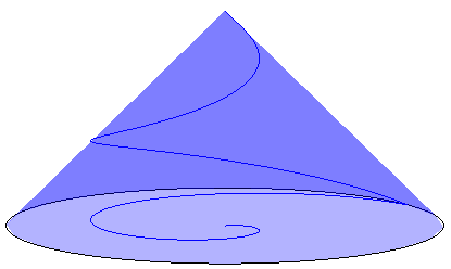
Mountain Path

At time $t$, the elevation reached is given by the composite function $$z=f(u(t),v(t))=:g(t).$$ The derivative of the function $g(t)$ tells us how fast we are climbing up the mountain, how fast our height is changing. To compute that we need a chain rule for the derivative of composite functions were one of the function (the outer one in this case) is bivariate.

Example 7.14 Let us go back to the mountain climbing example. Assume that the mountain elevation is given by $z=f(x,y)=1-\sqrt{x^2+y^2}$ for $x^2+y^2 \le 1$. This is a cone, with the vertex on $(0,0,1)$, the base being the unit disk, as in the picture above. Further, assume that the trail followed is given by $x=u(t)=(1-t)\cos(2\pi t)$ and $y=v(t)=(1-t)\sin(2\pi t)$ for $t\in [0,1)$; notice that these are the parametric equations of a curve. Calculate the vertical speed.

Using the expressions defining $x$ and $y$ in the definition of $z$ we have: $$z=f(u(t),v(t))=f((1-t)\cos(2\pi t),(1-t)\sin(2\pi t))=1-\sqrt{(1-t)^2}=t.$$ Hence, rather simply in this case, we get $\frac{dz}{dt}=1$ and the vertical speed is constant.

By reading the example, you may have realised that we may think of a number of composition of functions. Here we will just consider two cases:

• composition of single-variable functions with a function of several variable: $$z=f(u(t),v(t)),$$
• composition of functions of several variable with a function of several variables $$z=f(u(s,t),v(s,t)).$$

We can calculate the rate of change of height in a different way (often more convenient that in the previous simple expample) using the following theorem.

Theorem 7.1 (Chain Rule I) If $z=f(x,y)$ has continuous first partial derivatives on an open set $U\subset{\mathbb R}^2$ and $x=u(t), y=v(t)$ are differentiable functions of $t$ whose range is contained in $U$ (so, whenever $(x,y)\in U$), then the composition function is differentiable in $t$ and $$\frac{dz}{dt}={ \partial z \over \partial x}\frac{dx}{dt}+{ \partial z \over \partial y}\frac{dy}{dt}. \tag{7.3}$$

Proof: The following in an informal justification but gets across the idea. We start with $$\begin{eqnarray*} {z(t+h)-z(t) \over h} & = & {f(x(t+h),y(t+h))-f(x(t),y(t)) \over h} \\ & = & \left ({f(x(t+h),y(t+h))-f(x(t),y(t+h)) \over h} \right ) \\ && \quad + \left ({f(x(t),y(t+h))-f(x(t),y(t)) \over h} \right )\\ & = & \left ( {f(x(t+h),y(t+h))-f(x(t),y(t+h)) \over x(t+h)-x(t)} \right ) \left ({x(t+h)-x(t) \over h}\right ) \\ && \quad + \left ( {f(x(t),y(t+h))-f(x(t),y(t)) \over y(t+h)-y(t)} \right ) \left ({y(t+h)-y(t) \over h} \right ). \end{eqnarray*}$$ If we now take limits as $h \rightarrow 0$, if $x(t)$ and $y(t)$ are differentiable, we get $$\lim_{h \rightarrow 0} {z(t+h)-z(t) \over h} = {\partial f \over \partial x} {dx \over dt} + {\partial f \over \partial y} {dy \over dt}. \quad \Box$$

Example 7.15 Let us go back to Example~7.14. This time we use the chain rule (7.3): $${\partial z \over \partial x}=-\frac{x}{\sqrt{x^2+y^2}}=-\cos(2\pi t),\qquad {\partial z \over \partial y}=-\frac{y}{\sqrt{x^2+y^2}}=-\sin(2\pi t),$$ and $$\frac{dx}{dt}=-\cos(2\pi t)-2\pi (1-t)\sin(2\pi t),\qquad \frac{dy}{dt}=-\sin(2\pi t)+2\pi (1-t)\sin(2\pi t).$$ Thus, $$\frac{dz}{dt}=\cos^2(2\pi t)+2\pi (1-t) \cos (2\pi t)\sin (2\pi t)+\sin^2(2\pi t)-2\pi (1-t) \cos (2\pi t)\sin (2\pi t)=1.$$ So, the vertical speed is constant, exaclty as we got in Example~7.14.

In the next theorem we have a more sophisticated chain rule when the functions $x$ and $y$ also depend on two variables. This is typical of the situation when we are making a change of variable (e.g. to polar coordinates $x=r \cos \theta$, $y=r \sin \theta$) and we want to explore changes in the function with respect to these variables.

Theorem 7.2 (Chain rule II) Let $z=f(x,y)$ have continuous first partial derivatives on an open set $U\subset {\mathbb R}^2$ and $x=u(s,t), y=v(s,t)$ be differentiable functions of $s$ and $t$ whose range is contained in $U$ (so, whenever $(x,y)\in U$). Then the composition function admits first partial derivatives in $s$, and $t$ and $$\begin{eqnarray*} {\partial z \over \partial s} & = & {\partial z \over \partial x}{\partial x \over \partial s}+{\partial z \over \partial y}{\partial y \over \partial s},\\ {\partial z \over \partial t} & = & {\partial z \over \partial x}{\partial x \over \partial t}+{\partial z \over \partial y}{\partial y \over \partial t}. \tag{7.4} \end{eqnarray*}$$

Proof: This is an easy consequence of Chain rule I applied to the partial derivatives of $z=f(x,y)$ with respect to $s$ and $t$.

Notice that (7.4) can be re-written in matrix form as follows: $$\left [ \begin{array}{c} {\partial z \over \partial s} \\ {\partial z \over \partial t} \end{array} \right ] = \left [ \begin{array}{cc} {\partial x \over \partial s} & {\partial y \over \partial s} \\ {\partial x \over \partial t} & {\partial y \over \partial t} \\ \end{array} \right ] \left [ \begin{array}{c} {\partial z \over \partial x} \\ {\partial z \over \partial y} \end{array} \right ].$$ The matrix in (7.4) is called the Jacobian matrix of the transformation $(s,t)\rightarrow (x(s,t),y(s,t))$.

Example 7.16 Calculate the Jacobian matrix of the transformation from polar to Cartesian variables.

The change of variables polar to cartesian coordinates is given by $$x(r,\theta)=r\cos (\theta), \quad y(r,\theta)=r\sin (\theta).$$ The Jacobian of the transformation $(r,\theta)\rightarrow (x(r,\theta),y(r,\theta))$ is given by $$\left [ \begin{array}{cc} {\partial x \over \partial r} & {\partial y \over \partial r} \\ {\partial x \over \partial \theta} & {\partial y \over \partial \theta} \\ \end{array} \right ] = \left [ \begin{array}{cc} \cos \theta & \sin \theta \\ -r \sin \theta & r \cos \theta \\ \end{array} \right ]$$

Sometimes, when, say, $y$ is function of $x$ and their relationship is given implicitly, it is possible to calculate the rate of change of $y$ with respect to $x$, that is to get $\displaystyle\frac{d y}{d x}$ without finding first the explicit dependence of $y$ with respect to $x$. This technique is called implicit differentiation and can be easily derived using the chain rule.

Theorem 7.3 (Implicit Differentiation) If $z=u(x,y)$ is continuously differentiable and $y$ is a continuously differentiable function of $x$ that satisfies the equation $u(x,y(x))=0$, then at all points $z$ where ${\partial z \over \partial y} \neq 0$, $$\frac{d y}{d x}=-{{\partial z \over \partial x} \over {\partial z \over \partial y}}. \tag{7.5}$$

Proof: The proof is based on using the chain rule (7.3). In order to use the chain rule, we introduce a new variable $t$ and set $x=t$, in such a way that $$z=u(x(t),y(t))\quad\text{with}\quad x=t\quad\text{and}\quad y=y(t).$$ Now, since $z=u(x(t),y(t))=0$ for all $t$ by hypothesis, we have that $dz/dt=0$. Moreover, $dx/dt=1$ and $dy/dt=dy/dx$. Using these expression in @ref(eq:chainrule1} we get: $$\displaystyle 0={\partial z \over \partial x}+{\partial z \over \partial y}\frac{dy}{dx}.$$ Thus, for all those points $(x,y)$ for which ${\partial z \over \partial y}\neq 0$, we have (7.5).

Example 7.17 Suppose that $x^2+y^2=1$. Find $dy/dx$ using implicit differentiation and by direct calculation.

The function $z=u(x,y)=x^2+y^2-1$ defines the equation relating $x$ to $y$, that is $u(x,y)=0$. Thus, the implicit differentiation method gives: $$\displaystyle\frac{d y}{d x}=-\frac{2x}{2y}=-\frac{x}{y}.$$ To get the same result by direct calculation, we first need to find $y$ explicitly in function of $f$. Clearly, $y=\sqrt{1-x^2}$, at least for $x\in[-1,1]$. Then, $\frac{d y}{d x}=-\frac{x}{\sqrt{1-x^2}}$, which coincides with the previous result if you consider that $y=\sqrt{1-x^2}$.

7.5.1 Test yourself