Chapter 6 Differential Equations

6.1 Introduction

Differential equations arise nearly every time we try to model real world phenomena using mathematics. We recall that the derivative measures the of one quantity with regards to another. Newton’s second law says:

The rate of change of momentum of a body is equal to the applied external force.

The momentum of a body is the product of the mass $m$ and the velocity $v$ (in one dimension). Thus, if a body is experiencing a force $F$ then Newton’s law can be written mathematically as $${d \over dt} (mv) = F.$$ Thus we get an equation involving differentiation, and such an equation we call a differential equation. You have already met simple differential equations of the form $${df \over dt} = g(t), \tag{6.1}$$ for then the answer is $$f(t) = f(a)+\int_a^t g(x) dx.$$ It is important that we know the value of $f$ at some point, or else we cannot exactly say what $f$ is. We need a constant of integration. Below we have a picture where we can see that all these functions have the same derivative, so to choose which is the right one for our situation we have to know a point through which the function goes.

Definition 6.1 The solution where constants are not specified is called the general solution. The known value of $f$ is called an initial condition if our problem is a time-related problem, such as with Newton’s law. If the known value is a spatial value we call it a boundary condition. You have covered equations of type (6.1) in A level, and so we will not worry about these here.

Here is a web page with more examples of differential equations Differential equations at Mathisfun.com

6.1.1 The cultural heritage of mathematics

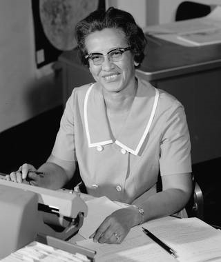
Katherine Johnson (1918 – 2020)

In 1962, the United States decided to send people to the Moon. Getting to and from the Moon would take a lot of work. Katherine studied how to use geometry for space travel. She figured out the paths for the spacecraft to orbit (go around) Earth and to land on the Moon. NASA used Katherine’s math, and it worked.
https://www.nasa.gov/audience/forstudents/k-4/stories/nasa-knows/who-was-katherine-johnson-k4

The paths that bodies take under gravitational attraction are the so-called conic sections.

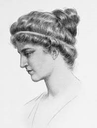
Hypatia (370-415)

Hypatia was known more for the work she did in mathematics than in astronomy, primarily for her work on the ideas of conic sections introduced by Apollonius. She edited the work On the Conics of Apollonius, which divided cones into different parts by a plane. This concept developed the ideas of hyperbolas, parabolas, and ellipses.
https://www.agnesscott.edu/lriddle/women/hypatia.htm

6.2 Separable equations

The next most straightforward sort of differential equation that we can solve is one of the form $${d y \over dx} = f(x) g(y), \tag{6.2}$$ for then we can write $$\int {dy \over g(y)} = \int f(x) dx.$$ We still need a boundary condition (we will assume that $x$ and $y$ are spatial variables here). We can integrate both of these in principle to get a solution.

Example 6.1

A projectile moving upwards is subject to a force due to gravity equal to $m g$ where $m$ is its mass, and $g$ is acceleration due to gravity. It is also slowed down by an air resistance which is equal to $mkv$, where $v$ is its speed and $k$ is some positive real constant which depends on the geometry of the projectile. The speed of the projectile at time $t=0$ is $u$ (this is the initial condition).

Newton’s second law says $${d \over dt} (mv) = -mkv-mg.$$ Since $m$ is constant in this equation (the projectile does not change mass as it flies) we can cancel $m$ from both sides above to get $${dv \over dt} = -(kv+g).$$ This is separable. Rearranging we have the equation $$\int {dv \over kv+g} = -\int dt.$$ Integrating both sides we have $${1 \over k} \log(kv+g) = -t+C,$$ where $C$ is a constant of integration that we find using the initial condition. When $t=0$ $v=u$ so that $${1 \over k} \log(ku+g) = C.$$ Thus $${1 \over k} \log(kv+g) = -t+{1 \over k} \log(ku+g).$$ Rearranging the above equation we have $$\begin{eqnarray*} t & = & {1 \over k} (\log(ku+g)-\log(kv+g)) \\ & = & {1 \over k} \log \left ( {ku+g\over kv+g } \right ). \end{eqnarray*}$$ Thus $$\exp(kt) = \left ( {ku+g\over kv+g } \right ).$$ Multiplying both sides by $kv+g$ we have $$kv \exp(kt)+g\exp(kt)=ku+g.$$ Hence $$kv \exp(kt) = ku+g(1-\exp(kt)),$$ so that $$v = u\exp(-kt)+{g \over k}(\exp(-kt)-1).$$

Remark. Check that this solves the original equation.

You can find more examples of separable equations and their solutions at Math24.net.

Example 6.2 Find the general solution of the separable differential equation $$y'=y(1-y).$$

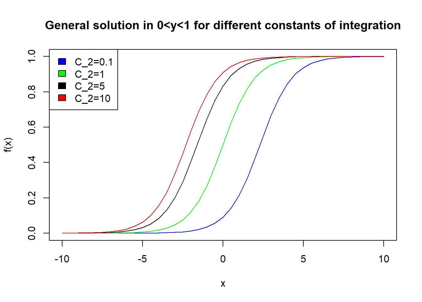
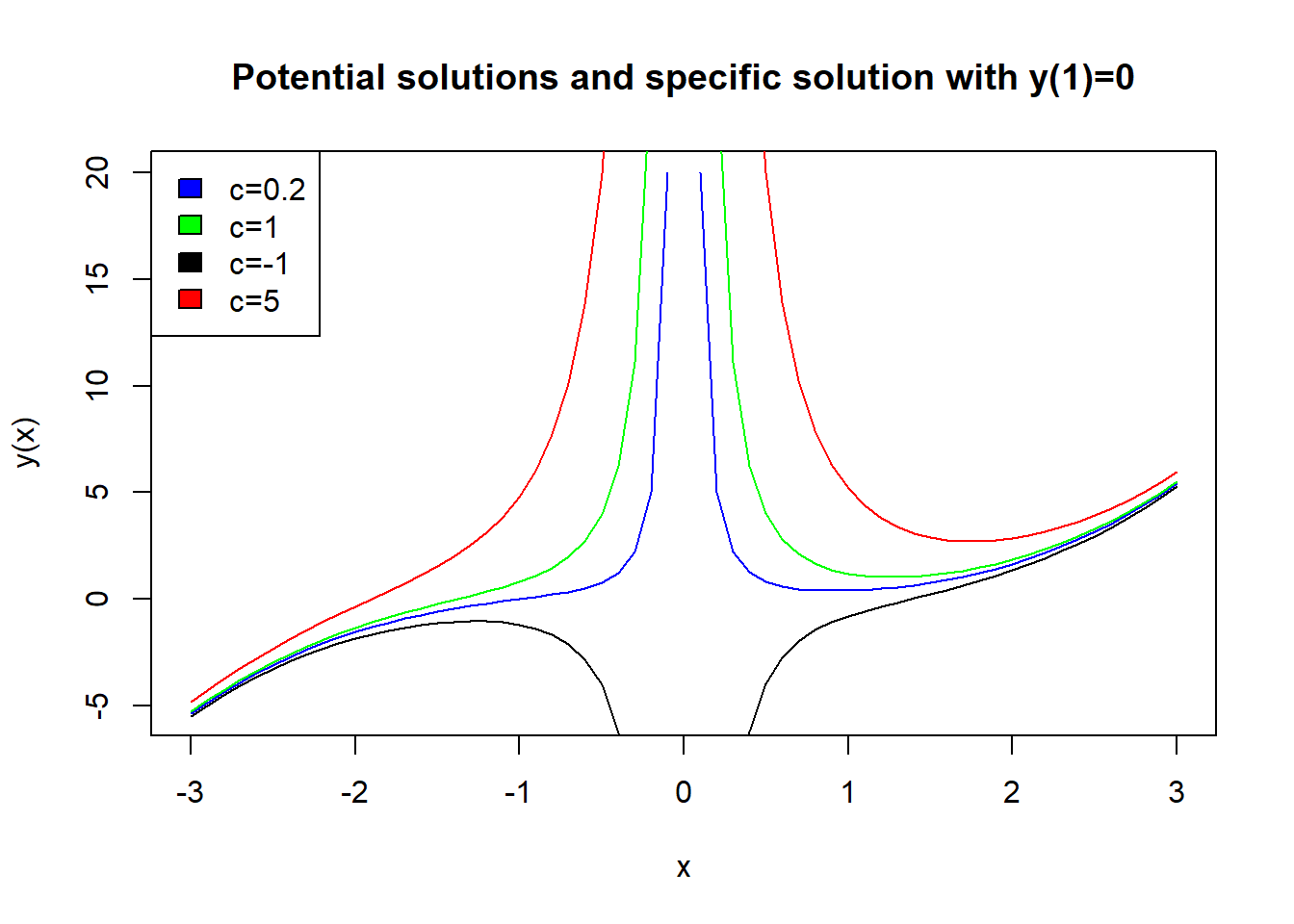
The equation is separable with $f(x)=1$ and $g(y)=y(1-y)$. Now $g(y)=0$ if and only if $y=0$ or $y=1$. So the equation can be solved by separating variables in the three intervals $y<0$, $0<y<1)$, and $y>1$. On any such interval, we have: $$\int \frac{dy}{y(1-y)}=\int dx+C_1,$$ with $C_1 \in {\mathbb R}$. This means that $$\int \left(\frac{1}{y}+\frac{1}{1-y}\right)dy=\int dx+C_1.$$ Therefore $$\ln |y|-\ln |1-y|=x+C_1 \; \Rightarrow \; \ln \left|\frac{y}{1-y}\right|=x+C_1,$$ and taking the exponential of both sides we have $$\left|\frac{y}{1-y}\right|=\exp(x+C_1)=\exp(C_1)\exp(x).$$ Since $C_1$ is constant, $\exp(C_1)>0$ is also constant. Let us call this $C_2$. Then, $$\left|\frac{y}{1-y}\right|=C_2\exp(x).$$ Now, $y/(1-y)$ is positve if $0<y<1$. In this case $$\left|\frac{y}{1-y}\right|=\frac{y}{1-y}=C_2\exp(x),$$ so that $$y=\frac{C_2\exp(x)}{C_2\exp(x)+1}=\frac{\exp(x)}{\exp(x)+1/C_2},\quad C_2>0.$$

Now $y/(1-y)$ is negative if $y<0$ or $y>1$. In this case
$$\left|\frac{y}{1-y}\right|=-\frac{y}{1-y}=C_2\exp(x),$$ so that $$y=\frac{C_2\exp(x)}{C_2\exp(x)-1}=\frac{\exp(x)}{\exp(x)-1/C_2}\quad C_2>0.$$ Now, if $\exp(x)>1/C_2$, i.e. $x>-\log(C_2)$, then $y>1$, and if $x<\log(C_2)$, then $y<0$. Hence we will have a vertical aymptote in $y$ at $x=-\log(C_2)$.

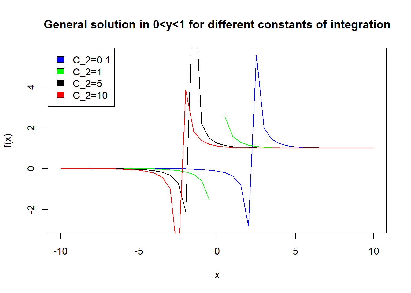
Remark IN the picture above you can see where the asymptotes are by the wierd jum in the graph. I have left this in, so that you can see how the solution changes from negative to greater than 1 as we move through $-\log(C_2)$. The situation seen with the previous example is typical of separable equations. You always need to examine the case $g(y)=0$ separately. Notice that if $g(y)=0$ then $y'=0$ thanks to the differential Equation (6.2). So the values $y$ for which $g(y)=0$ are constant stationary solutions of the equation.

Definition 6.2 A stationary or equilibrium solution for a differential equation $y'=f(x) g(y)$ is any solution $y(x)= Constant$. The stationary solutions can be found by solving for $y$ the equation $g(y)=0$ .

We can get a qualitative (behavioural) understanding of the solutions of these sort of equations by drawing the so-called direction fields.

Definition 6.3 A direction field on a region $S$ of the Cartesian plane is a map which assigns to each point of the region a line passing through that point. A curve ${\bf r} = {\bf r}(t)$ in the Cartesian plane is an integral curve of a direction field if its tangent lines coincide exactly with the lines of the direction field along the curve.

The lines of a direction field can be thought of as tangents to hypothetical curves. The idea of a tangent is closely bound up with the idea of slope (a.k.a. derivative). So instead of thinking of the lines in a direction field, we can think of the slope of the lines. (We allow infinite slope here.) And slope is given by a number.

So on the $(x,y)$-plane, we can identify a direction field with a function $f(x,y)$. And the idea of slope leads us to the equation $\frac{dy}{dx} =g(x,y)$.

Hence, the integral curves for the direction field correspond exactly to the solutions to this differential equation.

Example 6.3 Sketch the direction field for the equation $y'=y(1-y)$.

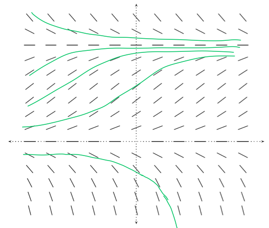We have $g(x,y)=y(1-y)$. We have seen already in Example 6.2 that $y=0$ and $y=1$ corresponding to zero rate of change (slope is horizontal) are stationary solutions. For $y<0$ and $y>1$ we have $g(x,y)<0$ (negative slope) and for $0<y<1$ we have $g(x,y)>0$ (positive slope). Thus qualitatively we can depict the equation’s direction fields as in the figure below. Direction fields and sketches of a few integral curves for Example ??

6.2.1 Test yourself

6.2.1.1 Equations of the form ${dy \over dx} = a{x \over y}$ and ${dy \over dx} = a{y \over x}$

6.2.1.2 Equations of the form ${dy \over dx} = {1+y^2 \over a+bx}$

6.3 Linear first order equations

Definition 6.4 Linear first order differential equations are ones of the form $${d y \over dx} + p(x)y(x)=q(x).$$ They are called linear because $y$ turns up with a power of 1 on the right hand side. Actually the previous example is of this type too, but is more easily solvable as a separable equation.

The main idea behind solving these equations is to rearrange the equation into $${d y \over dx} + p(x)y(x) = q(x), \tag{6.3}$$ and to try to turn the left hand side into the derivative of a product.

Recall that $${d \over dx} (I(x) y(x)) = I(x){dy \over dx}+y(x){dI \over dx}.$$ Multiply (6.3) by $I(x)$ (we use $I$ because this is going to be called the integrating factor) and then try to make it look like the equation above. Multiplying by $I(x)$ gives $$I(x) {d y \over dx} + I(x) p(x)y(x) = I(x)q(x)$$ We want $$I(x) {d y \over dx} + I(x) p(x)y(x) \equiv I(x){dy \over dx}+y(x){dI \over dx}.$$ For this to be true we need $$I(x) p(x) = {dI \over dx}.$$ This is a separable equation: $$\int {dI \over I} = \int p(x) dx,$$ which we solve to give $$\log I = \int p(x) dx,$$ so that $$I(x) = \exp \left ( \int p(x) dx \right ). \tag{6.4}$$

Definition 6.5 The function
$$I(x) = \exp \left ( \int p(x) dx \right )$$ is called the integrating factor for the differential equation $${d y \over dx} + p(x)y(x) = q(x).$$

Thus we have the following theorem:

Theorem 6.1 (Integrating Factor) Suppose we have the linear differential equation $${dy \over dx} + p(x) y(x) =q(x).$$ Then if $I$ is given by Equation (6.4) we can rewrite the equation above as $${d \over dx} (I(x) y(x)) = I(x) q(x).$$ The general solution of this differential equation is $$y(x) = {C \over I(x)}+{\int I(x) q(x) dx \over I(x)},$$ where $C$ is an arbitrary constant of integration.

Example 6.4 Let us try this out with Example 6.2. The equation we had was $${d v \over dt} = -kv-g.$$

We rearrange the last equation to get it into our standard form $${d v \over dt} +kv = -g.$$ which is a linear differential equation for $v$. The function $p(x)=k$ and $q(x)=-g$. Hence $$I(t)=\exp(\int (k) dt) = \exp(kt).$$ Then $${d \over dt} (\exp(kt)v) = k\exp(kt)v+\exp(kt){d v \over dx}=\exp(kt)\left ( {d v \over dt}+kv \right ) = -g \exp(kt).$$ If we integrate both sides we have $$\exp(kt)v = -{g \over k} \exp(kt) + C,$$ where $c$ is a constant of integration. The general solution (multiple both sides by $\exp(-kt)$) is $$v=-{g \over k}+C\exp(-kt).$$ We now use the initial condition that $v=u$ when $t=0$ to give $$u=-{g \over k}+C,$$ in other words $$C=u+{g \over k}.$$ Dividing both sides by $\exp(kt)$ we get $$v=u\exp(-kt)+{g \over k}(1-\exp(-kt)),$$ which is the same result as before.

Example 6.5 Solve the differential equation $${d y \over dx} + {2y \over x} = x^2,$$ where $y(1)=0$.

In this case the integrating factor is $$I(x) = \exp \left (\int {2 \over x} dx \right ) = \exp (2 \log x)=\exp (\log x^2)=x^2.$$ So $${d \over dx} (x^2 y) = x^2 {dy \over dx} + 2xy = x^2 \left ({dy \over dx} + 2{y \over x} \right )=x^2 (x^2) = x^4.$$ Hence $$x^2 y = {x^5 \over 5} + C,$$ where $C$ is a constant of integration. Thus we have a general solution $$y={x^3 \over 5} + {C \over x^2}.$$ We now use the boundary condition $y(1)=0$ to find a particular solution, giving $C=-1/5$.

You can find more examples of linear first order differential equations at math24.net.

6.3.1 Test yourself

6.4 Homogeneous equations

Definition 6.6 Homogeneous differential equations are equations of the form $${d y \over dx} = f \left ( {y \over x} \right ).$$

In this case we put $v=y/x$ so that $y=vx$. Then $${d y \over dx} = {d \over dx} (vx) = v + x {d v \over dx} = f(v).$$ Hence we have a separable equation $$\int {dv \over f(v)-v} = \int {dx \over x} = \log(|x|).$$ We can solve this if we can integrate the left hand side.

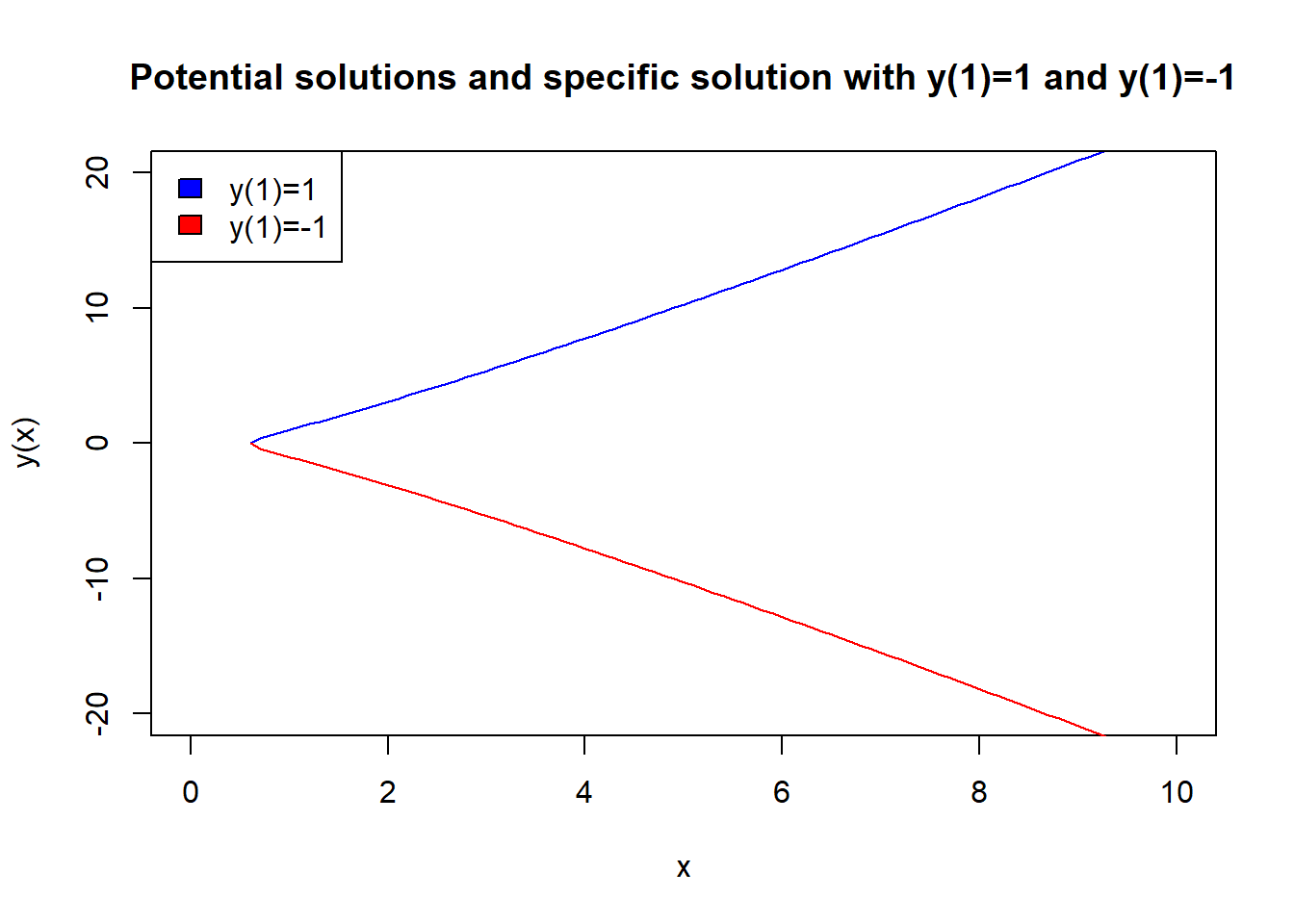
Example 6.6 Find the general solution of the differential equation $${d y \over dx} = {x^2 + y^2 \over xy}.$$

If we divide top and bottom by $x^2$ on the right hand side we get $${d y \over dx} = {1 + (y/x)^2 \over (y/x)}.$$ In this case the function $f(v)=(1+v^2)/v=1/v+v$. If we make the change of variable $y/x=v$, we have $$x{dv \over dx}+v={1+v^2 \over v}.$$ Rearranging this we get $$x{dv \over dx}={1\over v}+v-v = {1\over v}.$$ Hence $$\int v dv = \int {dx \over x}$$ so that $${v^2 \over 2} = \log|x|+C=\log A|x|,$$ where $A=e^C>0$. Therefore $$v= \pm \sqrt {2\log Ax},$$ where $A$ is an arbitrary positive constant of integration. In order for this to make sense we require that$2 \log A|x|>0$, so that $|x|>1/A$. However $v=y/x$, so that $$y= \pm x\sqrt {2\log A|x|}, \quad |x|>1/A,$$ is the general solution of the differential equation. We will choose a solution branch depending on where the initial condition is. For instance, $y(x)>0$ for positive $x$ then we have to choose the positive square root. But if $y(x)<0$ for positive $x$ we have to choose the negative square root. In the picture below we plot solutions where $y(1)=1$ (blue) and $y(1)=-1$ (red).

You can find more examples of homogeneous equations and their solutions at Math24.net

6.5 Second order linear differential equations with constant coefficients

Definition 6.7 A second order linear differential equation with constant coefficients is one of the form $$a{d^2 y \over dx^2} + b {d y \over dx}+cy=g(x),$$ where $a,b,c \in \mathbb{R}$ and $g(x)$ is a function of $x$.

The most well-known example of a second order equation with constant coefficients is the harmonic oscillator. In this equation we use Newtons’ second law, but use the fact that the velocity is the rate of change of the position of an object. So we have for acceleration $a$, velocity $v$ and displacement $x$, the following relationships $$a = {d v \over dt} = {d^2 x \over dt^2},$$ and $$v={dx \over dt}.$$

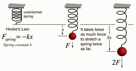
Hooke’s Law for modelling the motion of a spring

For a spring we have Hooke’s Law which says that if we extend a spring by an amount $x$ from its natural resting position, then the force of resistance to extension of the spring is $-kx$, where $k$ is a constant called the stiffness of the spring.

Thus, if we have a mass $m$ on a spring then the downward force will be $mg$ and the upward force due to the tension in the spring when extended distance $l$ will be $kl$. If $kl=mg$ then we will have no net force acting and the mass can be stationary. If we extend the spring by a further small distance $x$ and let it go then it will move upwards due to the excess tension in the spring over the weight. The equation of motion is $${d \over dt} (mv) = -k(l+x)+mg.$$ Since $kl=mg$ we get the equation $$m{dv \over dt} = -kx.$$ Substituting $v={dx \over dt}$ we obtain the equation $${d^2 x \over dt^2} = -{k \over m} x. \tag{6.5}$$ This is a famous differential equation called the equation of simple harmonic motion. This is an example of a second order linear differential equation with constant coefficients. Here is an explanation from a man with an American accent.

We solve equations like these by using the property of the exponential function that we discovered earlier - that these are eigenfunctions of the differentiation operator. We try a solution of the type $$x(t)=A \exp(\lambda t),$$ for some $\lambda$. Let us substitute this into our differential equation and see what happens.

Now $${d x \over dt} = A \lambda \exp(\lambda t),$$ and $${d^2 x \over dt^2} = A \lambda^2 \exp(\lambda t).$$ Substituting this into (6.5) we get $$A \lambda^2 \exp(\lambda t) = -{k \over m} (A \exp(\lambda t)).$$ Cancelling $A \exp(\lambda t) \neq 0$, we obtain $$\lambda^2 = -{k \over m}.$$ The solution of this equation is $$\lambda^2 = \pm i \sqrt{{k \over m}}.$$ Therefore the solution of the differential equation is $$x=A \exp \left ( i \sqrt{{k \over m}} \right )+B \exp \left ( -i \sqrt{{k \over m}} \right ),$$ for arbitrary constant $A, B$ (to be determined by initial conditions). Using the equations $$\exp(i \theta) = \cos \theta + i \sin \theta,$$ we can rewrite this as $$\begin{eqnarray*} x & = & A \left [ \cos \left (\sqrt{{k \over m}} \right )+i \sin \left (\sqrt{{k \over m}} \right ) \right ] + B \left [\cos \left ( -\sqrt{{k \over m}} \right )+i \sin \left ( -\sqrt{{k \over m}} \right ) \right ]\\ & = & A \left [ \cos \left (\sqrt{{k \over m}} \right )+i \sin \left (\sqrt{{k \over m}} \right ) \right ] + B \left [\cos \left ( \sqrt{{k \over m}} \right )-i \sin \left (\sqrt{{k \over m}} \right ) \right ] \\ & = & (A+B) \cos \left (\sqrt{{k \over m}} \right ) + i(A-B)\sin \left ( -\sqrt{{k \over m}} \right ). \end{eqnarray*}$$ So we see we have two different solution $\cos \left (\sqrt{{k \over m}} \right )$ and $\sin \left (\sqrt{{k \over m}} \right )$, and the constants $A+B$ and $i(A-B)$ depend on the boundary conditions.

Remark. You should check that these two functions satisfy the original differential equation. They are as it is impossible to make a combination of them (except the zero combination) identically equal to 0.

More generally we may have a second order differential equation of the following form $$a {d^2 y \over dx^2}+b{d y \over dx}+cy = g(x).$$ It is easiest in the first instance if we assume $g(x)=0$. Such an equation is called a homogeneous differential equation. Then, if we follow the same strategy as above, trying a solution of the form $y=e^{\lambda x}$, we change the differential equation to the algebraic equation $$a \lambda^2+b \lambda+c=0.$$ This equation is called the auxiliary equation.

The solution of the auxiliary equation can be in three different forms depending on the sign of the discriminant $$b^2-4ac.$$

Case 1: The easy case: $b^2-4ac>0$. In this case the two roots of the auxiliary equation are real: $$\lambda_{\pm} = {-b\pm\sqrt{b^2-4ac} \over 2a},$$ and the general solution of the homogeneous equation is $$y=A\exp(\lambda_+ x)+B \exp(\lambda_- x),$$ where $A$ and $B$ are arbitrary real constants, which can be determined from boundary conditions.

Example 6.7 Find the general solution of the linear second order differential equation $${d^2 y \over dx^2}+3{d y \over dx}+2y=0.$$

The auxiliary equation is $$\lambda^2+3\lambda+2=0,$$ which has solutions $\lambda_1=-1$ and $\lambda_2=-2$. Hence the general solution to this differential equation is $$y=A\exp(-x)+B\exp(-2x).$$ Suppose that $y(0)=1$ and $y'(0)=0$. Then $$y(0)=A+B=1,$$ and $$y'(0)=-A-2B=0.$$ We can solve these simultaneous equations to get $A=2$ and $B=-1$, so that $$y=2\exp(-x)-\exp(-2x).$$

Case 2: $b^2-4ac=0$. In this case we have two equal roots, $\lambda=-b/(2a)$. Then we have a general solution of the form $$y=A\exp(\lambda x)+Bx \exp(\lambda x).$$ You should check that this is true.

Example 6.8 Find the general solution of the linear second order differential equation $${d^2 y \over dx^2}-2{d y \over dx}+y=0.$$ The auxiliary equation is $$\lambda^2-2\lambda+1=0,$$ which has solution $\lambda=1$. Hence the general solution to this differential equation is $$y=A\exp(x)+Bx\exp(x).$$ Suppose that $y(0)=2$ and $y'(0)=1$. Then $$y(0)=A=2,$$ and $$y'(0)=A+B=1,$$ so that $B=-1$. Hence the solution in this case is $$y=2\exp(x)-x\exp(x).$$

Case 3: $b^2<4ac$. In this case the solutions of the auxiliary equation are complex: $$\lambda_\pm = {-B \over 2A} \pm i{\sqrt{4ac-b^2} \over 2a} = \lambda_R \pm i \lambda_I,$$ where $\lambda_R = {-b \over 2a}$ and $\lambda_I={\sqrt{4ac-b^2} \over 2a}$. The general solution is then $$y=\exp(\lambda_R x) (A \cos (\lambda_I x)+B \sin (\lambda_I x)).$$ Again you should check that this is true.

Example 6.9 Find the general solution of the linear second order differential equation $${d^2 y \over dx^2}+2{d y \over dx}+3y=0.$$ The auxiliary equation is $$\lambda^2+2\lambda+3=0,$$ which has solution $\lambda=-1\pm i\sqrt{2}$. So $\lambda_R=-1$ and $\lambda_I=\sqrt{2}$. Hence the general solution to this differential equation is $$y=\exp(-x)(A \cos (\sqrt{2} x)+B\sin (\sqrt{2} x)).$$ Suppose that $y(0)=1$ and $y'(0)=0$. Then $$y(0)=A=1,$$ and $$y'(0)=-A+\sqrt{2}B=0,$$ so that $B=1/\sqrt{2}$. Hence the solution in this case is $$y=\exp(-x)\left (\cos (\sqrt{2} x)+{1 \over \sqrt{2}} \sin (\sqrt{2} x) \right ).$$

Video revising solution of second order differential equations

6.5.1 Test yourself

6.6 Challenge Yourself

1. Explore the solution of the Bernoulli equation $y'+p(x)y=q(x)y^n$, for $n \ge 0$.
2. In this question you are going to approximately solve the differential equation $y'=y$, $y(0)=2$, using the limit definition of differentiation. Let $h=0.1$. Find the approximate value of $y(h)$ using the approximation $${y(h)-y(0) \over h} = y'(0)=y(0),$$ where the second equation follows from the differential equation $y'=y$. Compare the approximate answer to the actual answer by analytically solving the differential equation. Now find approximate values at $ih$ for $i \ge 1$. What happens to the solution as $h \rightarrow 0$.
3. Can you find an approximation to ${d^2 y \over dx^2}$ at a point $a$ by using $y(a-h)$, $y(a)$ and $y(a+h)$. Suppose you know $y(a)$ and $y'(a)$. If you have a second order differential equation $${d^2 y \over dx^2}=y,$$ can you find $y(a-h)$ and $y(a+h)$?
4. Do some research into second order differential equations with a non-zero right hand side: $$A {d^2 y \over dx^2} + B{dy \over dx}+Cy = g(x).$$