8 Majorization Inequalities

8.1 Introduction

8.2 The AM/GM Inequality

8.2.1 Absolute Values

8.2.2 Absolute Values

Suppose the problem we have to solve is to minimize $$f(x)=\sum_{i=1}^nw_i|h_i(x)|$$ over $x\in\mathcal{X}.$ Here $h_i(x)$ is supposed to be differentiable. In statistics it typically is a residual, for instance $h_i(x)=y_i-z_i'x.$ Suppose, for the time being, that $h_i(x)\not= 0$. Then we have the majorization $$\sum_{i=1}^nw_i|h_i(x)|\leq \frac{1}{2}\sum_{i=1}^n\frac{w_i}{|h_i(y)|} (h^2_i(x)+h^2_i(y)),$$ and we must minimize $$g(x,y):=\sum_{i=1}^n\frac{w_i}{|h_i(y)|}h^2_i(x),$$ which is a weighted least squares problem.

The simplest case of this is the one-dimensional example is $h_i(x)=y_i-x$, which means we want to compute the weighted median. The algorithm is simply $$x^{(k+1)}=\frac{\sum_{i=1}^n u_i(x^{(k)})y_i}{\sum_{i=1}^n u_i(x^{(k)})},$$ where $$u_i(x)=\frac{w_i}{\mid y_i-x\mid}.$$

We have assumed, so far, in this example that $h_i(y)\not= 0$. If $h_i(y)=0$ at some point in the iterative process then the majorization function does not exist, and we cannot compute the upgrade. One easy way out of this problem is to minimize $$f_\epsilon(x)=\sum_{i=1}^nw_i\sqrt{h_i^2(x)+\epsilon^2}$$ for small values of $\epsilon$. Clearly if $\epsilon_1>\epsilon_2$ then $$\min_x f_{\epsilon_1}(x)=f_{\epsilon_1}(x_1)>f_{\epsilon_2}(x_1)\geq\min_x f_{\epsilon_2}(x).$$ It follows that

The function $f_\epsilon$ is differentiable. We find $$\mathcal{D}f_\epsilon(x)=\sum_{i=1}^n w_i\frac{h_i(x)}{\sqrt{h_i^2(x)+\epsilon^2}}\mathcal{D}h_i(x),$$ and $$\mathcal{D}^2f_\epsilon(x)=\sum_{i=1}^n w_i\frac{1}{\sqrt{h_i^2(x)+\epsilon^2}} \left\{\frac{\epsilon^2}{h_i^2(x)+\epsilon^2}\left(\mathcal{D}h_i(x)\right)^2+h_i(x)\mathcal{D}^2h_i(x)\right\}.$$ With obvious modifications the same formulas apply if $x$ is a vector of unknowns, for instance if $h(x)=y-Zx$.

By the implicit function theorem the function $x(\epsilon)$ defined by $\mathcal{D}f_\epsilon(x(\epsilon))=0$ is differentiable, with derivative $$\mathcal{D}x(\epsilon)=\epsilon\frac{\sum_{i=1}^nw_i\left[h_i^2(x(\epsilon))^2+\epsilon^2\right]^{-\frac32}h_i(x(\epsilon))\mathcal{D}h_i(x(\epsilon))}{\mathcal{D}^2f_\epsilon(x(\epsilon))}$$

For the weighted median the iterates are still the same weighted averages, but now with weights $$u_i(x,\epsilon)=\frac{w_i}{\sqrt{(y_i-x)^2+\epsilon^2}}.$$ Differentiating the algorithmic map gives the convergence ratio $$\kappa_\epsilon(x)\mathop{=}\limits^{\Delta}\frac{\sum_{i=1}^n u_i(x,\epsilon)\frac{(y_i-x)^2}{(y_i-x)^2+\epsilon^2}}{\sum_{i=1}^n u_i(x,\epsilon)}.$$ Clearly $$\min_i\frac{(y_i-x)^2}{(y_i-x)^2+\epsilon^2}\leq\kappa_\epsilon(x)\leq\max_i\frac{(y_i-x)^2}{(y_i-x)^2+\epsilon^2},$$ which implies $\kappa_\epsilon(x)< 1.$ If $y_i\not=x$ for all $i$, then $\lim_{\epsilon\rightarrow 0}\kappa_\epsilon(x)=1$ and convergence is asymptotically sublinear.

---

Insert mediJan.R Here

---

8.2.3 Gini Mean Difference

Alternatively, we can minimize the Gini Mean Difference of the $f_i(\theta).$ Now

$$\begin{multline*} \sum_{i=1}^n\sum_{j=1}^n\mid f_i(\theta)-f_j(\theta)\mid \leq\\ \sum_{i=1}^n\sum_{j=1}^n\frac{1}{\mid f_i(\xi)-f_j(\xi)\mid} (f_i(\theta)-f_j(\theta))^2 + \text{terms}, \end{multline*}$$

which can be rewritten as $$\cdots=\sum_{i=1}^n\sum_{j=1}^n w_{ij}(\xi)f_i(\theta)f_j(\theta)+\text{terms},$$ minimization of which is a weighted least squares problem.

8.2.4 Location Problems

The Fermat-Weber problem is to find a point $x\in\mathbb{R}^m$ such that the sum of the Euclidean distances to $m$ given points $y_1,\cdots,y_m$ is minimized. Thus our loss function is $$f(x)=\sum_{j=1}^m w_jd(x,y_j),$$ where the $w_j$ are positive weights. Other names are the single facility location problem or the spatial median problem.

An early iterative algorithm to solve the Fermat-Weber problem was proposed by Weiszfeld (1937). For a translation see Weiszfeld and Plastria (2009).

Here we show how to use the arithmetic mean-geometric mean inequality for majorization. Suppose our problem is to minimize $$f(X)=\sum_{i=1}^n\sum_{j=1}^n w_{ij}d_{ij}(X),$$ where the $w_{ij}$ are non-negative weights, and the $d_{ij}(X)$ are again Euclidean distances. This is a location problem. To make it interesting, we suppose that some of the points (facilities) are fixed, others are the variables we have to minimize over. Observe that this is a convex, but non-differentiable, optimization problem.

We use the AM-GM inequality in the form $$d_{ij}(X)d_{ij}(Y)\leq\frac{1}{2}(d_{ij}^2(X)+d_{ij}^2(Y)).$$ If $d_{ij}(Y)>0$ then $$d_{ij}(X)\leq\frac{1}{2}\frac{d_{ij}^2(X)+d_{ij}^2(Y)} {d_{ij}(Y)}.$$ Using the notation from Example a.a we now find $$\phi(X)\leq\frac{1}{2}(\hbox{tr }X'B(Y)X+\hbox{tr }Y'B(Y)Y),$$ which gives us a quadratic majorization.

If $X$ is partitioned into $X_1$ and $X_2,$ with rows which are fixed and rows which are to be determined (facilities which have to be located), and $B$ is partitioned correspondingly, then the algorithm we find is $$X_2^{(k+1)}=B_{22}(X^{(k)})^{-1}B_{21}(X^{(k)})X_1.$$

8.2.5 The Lasso and the Bridge

8.3 Polar Norms and the Cauchy-Schwarz Inequality

8.3.1 Rayleigh Quotient

Rewrite for minimizing 02/22/15, by maximizing x’Bx over x’Ax=1.

We go back to maximizing the Rayleigh quotient $$\lambda(x)=\frac{x'Ax}{x'Bx},$$ where we now assume that both $A$ and $B$ are positive definite. Maximizing $\lambda$ is equivalent to maximizing $\sqrt{x'Ax}$ on the condition that $\sqrt{x'Bx}=1$. By Cauchy-Schwartz $$\sqrt{x'Ax}\geq\frac{1}{\sqrt{y'Ay}}x'Ay,$$ and thus for the majorization we maximize $x'Ax$ over $x'Bx=1.$ This defines an algorithmic map which sets the update of $x$ proportional to $B^{-1}Ax,$ i.e. we have a shown global convergence of the power method to compute the largest generalized eigenvalue.

We can also establish the linear convergence rate quite easily, using Ostrowski (1966). For definiteness we normalize in each iteration, and set $$\mathcal{A}(\omega)=\frac{B^{-1}A\omega}{\|B^{-1}A\omega\|}.$$ At a point $\omega$ which has $B^{-1}A\omega=\lambda_1\omega,$ and $\omega'\omega=1$ we have $$\mathcal{M}(\omega)=\frac{1}{\lambda_1}(I-\omega\omega')B^{-1}A.$$ It follows that $\mathcal{M}$ has eigenvalues $0$ and $\frac{\lambda_s}{\lambda_1}$, with $\lambda_s$ the ``remaining’’ eigenvalues of $B^{-1}A.$ Thus if $\lambda_1$ is the largest eigenvalue, we find a linear rate of $\rho=\frac{\lambda_1}{\lambda_2}.$

There are several things in this analysis which may go wrong, and they are all quite instructive.

8.3.2 The Majorization Method for MDS

The first is an algorithm for multidimensional scaling, developed by De Leeuw (1977). We want to minimize $$\sigma(X)=\frac{1}{2}\sum_{i=1}^m\sum_{j=1}^m w_{ij}(\delta_{ij}-d_{ij}(X))^2,$$ with $d_{ij}(X)$ again Euclidean distance, i.e. $$d_{ij}(X)=\sqrt{(x_i-x_j)'(x_i-x_j)}.ƒ$$ We suppose weights $w_{ij}$ and dissimilarities $\delta_{ij}$ are symmetric and hollow (zero diagonal), and satisfy $$\frac{1}{2}\sum_{i=1}^m\sum_{j=1}^m w_{ij}\delta_{ij}^2=1.$$ We now define the following objects $$\begin{align} \eta^2(X)&\mathop{=}\limits^{\Delta}\sum_{i=1}^m\sum_{j=1}^m w_{ij}d_{ij}(X)^2,\\ \rho(X)&\mathop{=}\limits^{\Delta}\sum_{i=1}^m\sum_{j=1}^m w_{ij}\delta_{ij}d_{ij}(X). \end{align}$$ Thus $$\sigma(X)=1-2\rho(X)+\frac{1}{2}\eta^2(X).$$ The next step is to use matrices. Let $$\begin{align} v_{ij}&= \begin{cases}-w_{ij}& \text{if $i\not= j,$}\\ \sum_{k\not=i}^m w_{ik}& \text{if $i=j$,} \end{cases}\\ b_{ij}(X)&= \begin{cases} -\frac{w_{ij}\delta_{ij}}{d_{ij}(X)}& \text{if $i\not= j,$}\\ \sum_{k\not=i}^m\frac{w_{ik}\delta_{ik}}{d_{ik}(X)}& \text{if $i=j$.} \end{cases} \end{align}$$ Now $$\sigma(X)=1-\hbox{tr}X'B(X)X+\frac{1}{2}\text{tr}X'VX.$$ By Cauchy-Schwarz, $$d_{ij}(X)\geq\frac{(x_i-x_j)'(y_i-y_j)}{d_{ij}(Y)},$$ which implies $$\hbox{tr}X'B(X)X\geq\hbox{tr}X'B(Y)Y.$$ Now let $$\overline X=V^+B(X)X.$$ This is called the Guttman-transform of a matrix $X.$ Using this transform we see that for all pairs of configurations $(X,Y)$ $$\begin{align} \sigma(X)&\leq 1-\hbox{tr }X'B(Y)Y+\frac{1}{2}\text{tr }X'VX=\\ &=1-\hbox{tr }XV\overline Y+\frac{1}{2}\text{tr }X'VX=\\ &=1-\frac{1}{2}\text{tr }\overline Y'V\overline Y+ \frac{1}{2}\text{tr }(X-\overline Y)'V(X-\overline Y), \end{align}$$

while for all configurations $$X$$ we have $$\sigma(X)=1-\frac{1}{2}\text{tr }\overline X'V\overline X+ \frac{1}{2}\text{tr }(X-\overline X)'V(X-\overline X).$$

8.4 Conjugates and Young’s Inequality

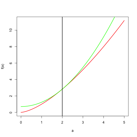
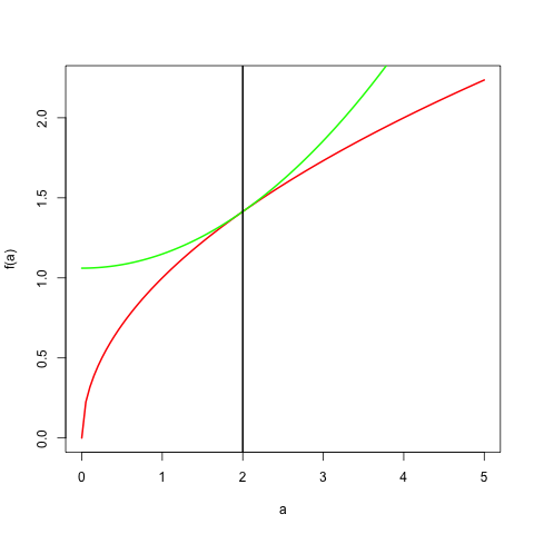
Example: Let $0<r<2$, $p=\frac{2}{r}$, and $q=\frac{2}{2-r}$. Then the previous result, applied to $x^r$ and $y^{2-r}$, becomes $$x^ry^{2-r}\leq\frac{r}{2}x^2+\frac{2-r}{2}y^2,$$ which provides us with a quadratic majorization for $x^r$ for all $0<r<2.$ We have equality if and only if $x=y$.

showMe <- function (b, r, up = 5) {
    a <- seq (0, up, length = 100)
    ar <- a ^ r
    plot (a, ar, type = "l", col = "RED",
          ylab="f(a)", lwd = 2)
    br <- (r * (a ^ 2)) / 2 + (((2 - r)  * (b ^ 2))/ 2)
    br <- br / (b ^ (2 - r))
    lines (a, br, col = "GREEN", lwd = 2)
    abline (v = b, lwd = 2)
}

Here is an example with $y=2$ and $r=1.5$.

One important application of these results is majorization of powers of Euclidean distances $(\sqrt{x'Ax})^r$ by quadratic forms. We find, for $0<r<2$, $$(\sqrt{x'Ax})^r\leq\frac{1} {(\sqrt{y'Ay})^{(2-r)}}\left\{\frac{r}{2}x'Ax+\frac{2-r}{2}y'Ay\right\}$$

8.4.1 Support Vector Machines