6 Distributions of random variables
In probability, we use the word “distribution” to refer to how all possible values of a random variable are distributed. This implies knowledge of how to calculate probabilities related to such random variable. In section 6.1, we define functions that describe the distribution of a random variable (PMF, PDF, and CDF). In sections 6.2 and 6.3, we look at two distributions that are encountered often in statistics and that are used to develop methods for statistical inference. More specifically, we will look at a discrete distribution (binomial) and a continuous distribution (normal).
6.1 PMFs, PDFs, and CDFs
From definition 5.2, a random variable is the assignment of a numerical outcome to a random process. We usually represent a random variable with a capital letter. A random variable can be discrete or continuous, depending on the values that it takes. For example, the number of heads in 2 coin flips is a discrete random variable because it can only take the values 0, 1, and 2. The time until the next earthquake is a continuous random variable because it can take any non-negative value.
Definition 6.1 The probability mass function (PMF)14 of a discrete random variable \(X\) is defined as \[f(k) = P(X = k)\] and it has the following properties:
- \(0\leq f(k) \leq 1\) (the probability must be within the interval [0,1]).
- \(\sum_k f(k) = 1\) (the sum of the probabilities of all outcomes in the sample space must be 1).
The PMF gives the probability that a discrete random variable takes a specific value. PMFs are only used for discrete random variables, while another type of function is used for continuous ones (see definition below).
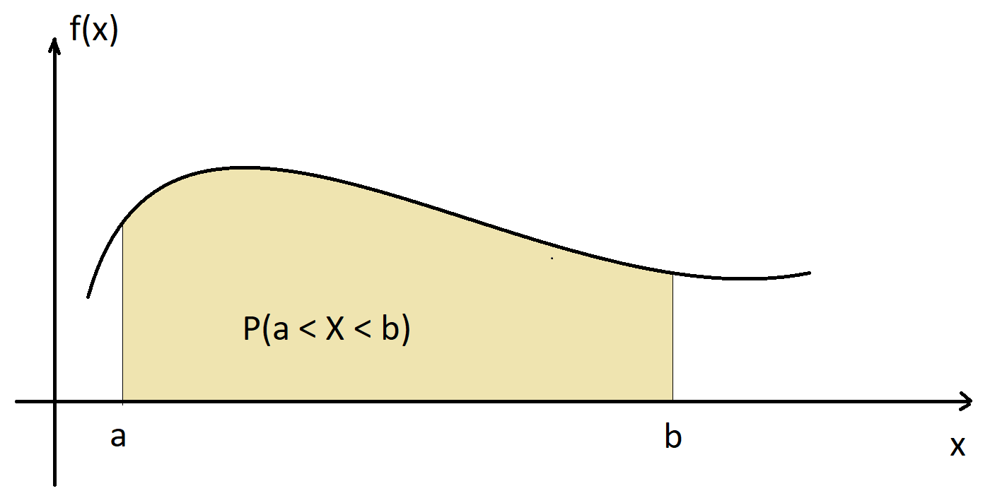
Definition 6.2 The probability density function (PDF) of a continuous random variable \(X\) is a function \(f:\mathbb{R}\rightarrow\mathbb{R}\) such that \(P(a \leq X \leq b)\) is the area under the graph of \(f\) between \(a\) and \(b\), as illustrated in the figure below. In mathematical symbols, \[P(a \leq X \leq b) = \int_a^b f(x)dx.\] The PDF satisfies:
- \(f(x)\geq 0\).
- \(\int_{-\infty}^{\infty} f(x) dx = 1.\) That is, the total area under \(f(x)\) is 1.
We can think of the PDF as a smooth histogram with very slim bins, where the areas of the bins sum to 1. From definition 6.2, the probability that a continuous random variable takes one specific value is zero because the area under any function at one specific point is zero. This is the reason why it does not make sense to use PMFs for continuous random variables.
The PMF and PDF are functions whose goals are to calculate probabilities of random processes, but only the output of a PMF gives a probability. The output of a PDF is not a probability - we need to find an area to get a probability.
Example 6.1 Suppose that the Old Faithful erupts every 91 minutes exactly (we know it’s not exact, but for the sake of this example let’s suppose it is). I’m on a trip and have only budgeted 20 minutes to observe it. What’s the probability that I observe it erupt?
Let \(T\) be the time after my arrival (in minutes) in which the Old Faithful erupts. Notice that \(T\) is a continuous random variable that can take values in the interval \((0,91]\). That is, the sample space of this random process is \((0,91]\). I’m hopping the eruption will happen within the interval \((0,20]\), so I want to know \(P(T\leq 20).\) This calculation is done as follows:
\[P(T \leq 20) = \frac{\mbox{length of interval of interest}}{\mbox{length of total interval}} = \frac{20-0}{91-0} = 0.22.\] That is, there’s a 22% chance that I will observe the Old Faithful erupt.
Now what is the probability that I observe it erupt exactly 19.2 minutes after I arrive? In this case,
\[P(19.2 \leq T \leq 19.2) = \frac{\mbox{length of interval of interest}}{\mbox{length of total interval}} = \frac{19.2-19.2}{91-0} = \frac{0}{91} = 0,\]
which is an impossible event. Finally, what is the probability that I observe it erupt within my last minute there? In this case,
\[P(19 \leq T \leq 20) = \frac{\mbox{length of interval of interest}}{\mbox{length of total interval}} = \frac{20-19}{91-0} = \frac{1}{91} = 0.01.\]
Since \(P(T=a)=0\) for any time \(a\), we can opt to use \(\leq\) or \(<\) to write the probabilities of \(T\) being within two numbers. Further, from the examples above, it follows that the PDF for \(T\) is the following function:
\[ f(x) = \left\{ \begin{array}{l} \frac{1}{91}, \quad \mbox{if } 0\leq x \leq 91,\\ 0, \quad \mbox{otherwise.} \end{array} \right. \]
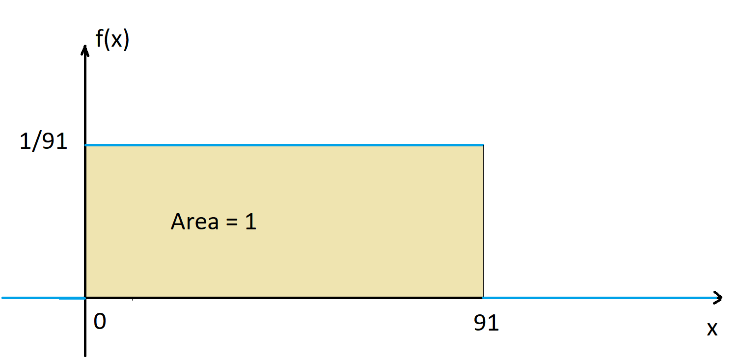
Random variables where the PDF is a horizontal line within two values are called a continuous uniform random variable.
Example 6.2 Let \(H\) be the number of heads in two coin flips. The possible outcomes \(H\) and their probabilities are: \[\begin{eqnarray} P(H=0) &=& P(TT) = \frac{1}{4},\\ P(H=1) &=& P(HT \cup TH) = \frac{1}{2},\\ P(H=2) &=& P(HH) = \frac{1}{4}. \end{eqnarray}\] Therefore, the PMF for \(H\) is \[ f(k) = \left\{ \begin{array}{l} \frac{1}{4}, \quad k = 0,\\ \frac{1}{2}, \quad k = 1,\\ \frac{1}{4}, \quad k = 2,\\ 0, \quad \mbox{otherwise.} \end{array} \right. \]
Definition 6.3 The cummulative distribution function (CDF) of a discrete or continuous random variable is the function given by \(F(x) = P(X\leq x).\)
In example 6.2 above,
\[ F(x) = \left\{ \begin{array}{l} 0, \quad x<0,\\ \frac{1}{4}, \quad 0\leq x < 1,\\ \frac{3}{4}, \quad 1\leq x < 2,\\ 1, \quad x \geq 2. \end{array} \right. \]
In example 6.1 (Old Faithful), the CDF is
\[ F(x) = \left\{ \begin{array}{l} 0, \quad x<0,\\ \frac{x-0}{91-0} = \frac{x}{91}, \quad 0\leq x < 91,\\ 1, \quad x \geq 91. \end{array} \right. \]
Example 6.3 Consider a continuous random variable whose PDF is displayed below (this is called a triangular random variable).
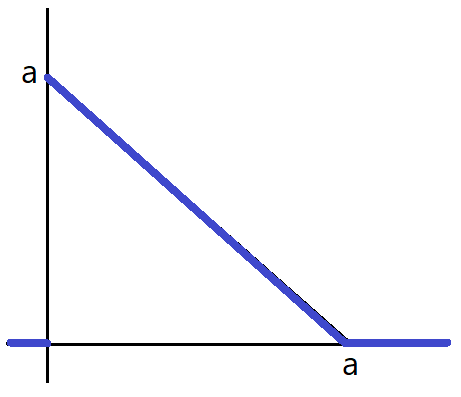
What should be the value of “a” so that this is a valid PDF?
Write the formula for the PDF.
What is the CDF of this random variable?
Answers:
To be a PDF, the area between the PDF and the x-axis must be 1. This means that \(a^2/2 = 1\), which gives \(a = \sqrt{2}\).
The formula for the PDF is: \[ f(x) = \left\{ \begin{array}{l} -x + \sqrt{2}, \quad 0\leq x < \sqrt{2},\\ 0, \quad \mbox{otherwise}. \end{array} \right. \]
To find the CDF \(F(x)\), we compute the grey area below, for all possible values of \(x\).
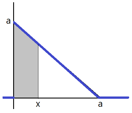
When \(x < 0\), the area is zero.
When \(0 \leq x < \sqrt{2},\) the area is \(\int_0^x (-u + \sqrt{2})du = -\frac{x^2}{2} + \sqrt{2}x.\)
When \(x \geq \sqrt{2},\) he area is 1.
This gives the CDF:
\[ F(x) = \left\{ \begin{array}{l} 0, \quad x < 0,\\ -\frac{x^2}{2} + \sqrt{2}x, \quad 0 \leq x < \sqrt{2},\\ 1, \quad x \geq \sqrt{2}. \end{array} \right. \]
6.2 Binomial distribution
Before describing the binomial distribution, we define one of the simplest discrete random variables: the Bernoulli random variable.
A Bernoulli random variable \(X\) is an indicator random variable, that is, it only takes the values 1 (“success”) and 0 (“failure”). The probability of \(X=1\) is denoted by \(p\). Random experiments that lead to Bernoulli random variables are called Bernoulli trials. For example, the number of heads in one coin flip is a Bernoulli random variable and the coin flip is a Bernoulli trial.
A random variable \(Y\) is called a binomial random variable if it counts how many outcomes in \(n\) independent Bernoulli trials are a “success.”
Notation: We use the notation \(Y \sim Binom(n,p)\) to say that \(Y\) has the distribution of a binomial random variable with \(n\) Bernoulli trials and probability of success \(p\).
For example, the random variable \(H\) described in example 6.2 is a binomial random variable because it counts the number of heads in 2 coin flips. In this example, the Bernoulli trials are the 2 independent coin flips, and “heads” is the characteristic of interest (success). In example 6.2, it was feasible to calculate the probabilities of all possible outcomes and write the PMF. What if \(H\) was the number of heads in 20 coin flips? We could still list all possible outcomes and their probabilities, but it it turns out that there is an easy-to-use formula for the PMF of a binomial random variable.
The PMF of a binomial random variable \(Y\) is given by
\[ f(k) = P(Y = k) = {n \choose k}p^k(1-p)^{n-k}. \]
The expression \({n \choose k}\) is equal to \(\frac{n!}{k!(n-k)!}\).
The factorial of a number \(k\) is the product of \(k\) with all natural numbers less than \(k\). For example, \(4! = 4\times 3\times 2\times 1.\) It is the number of ways in which one can list \(k\) distinct objects. The factorial of 0 is 1, that is, \(0!=1\). This implies that \({n \choose 0} = {n \choose n} = 1.\)
In the formula above, \(n\) is the number of independent Bernoulli trials and \(p\) is the probability of success in each trial. The values \(n\) and \(p\) are called parameters of the binomial distribution, so when describing a binomial random variable, these values should be provided.
Example 6.4 Let \(H\) be the number of heads in 20 coin flips. Then \(H\) is a binomial random variable with \(n=20\) and \(p=0.5\). The probability of observing exactly 5 heads is
\[ P(Y = 5) = {20 \choose 5}0.5^5(1-0.5)^{20-5} = \frac{20!}{5!15!} 0.5^5 0.5^{15} = 0.01479. \]
In R, the binomial PMF is the function dbinom. More specifically, dbinom(k, n, p) = \({n \choose k}p^k(1-p)^{n-k}.\) So the probability calulation for example 6.4 can be done by running the command:
## [1] 0.01478577Example 6.5 What if we were interested in knowing the probability of obtaining at least 2 heads in 20 coin flips? In this case, we want to know \(P(H \geq 2)\). There are several ways to calculate this probability, some being unnecessarily tedious. For example, we could calculate
\[P(H\geq 2) = P(H=2)+P(H=3) + \cdots + P(H=20) = \cdots\]
or we could use the complement of \(H\geq 2\) (see section 5.1) and calculate
\[\begin{eqnarray} P(H\geq 2) &=& 1 - P(H < 2) = 1 - (P(H=0)+P(H=1)) \\ &=& 1-(1\times 0.5^0 0.5^{20} + 20\times 0.5^1 0.5^{19}) = 0.99998. \end{eqnarray}\]
R also has functions for the CDF of a random variable. For the binomial random variable \(Y\) with parameters \(n\) and \(p\), the command pbinom(k, n, p) calculates \(P(Y\leq k).\)
In example 6.5, the probability \(P(Y<2)\) can also be written as \(P(Y\leq 1)\) because \(Y\) takes only values in the natural numbers. So we can use pbinom to carry out the calculation \(P(H\geq 2) = 1 - P(H \leq 1):\)
## [1] 0.99998Notice that pbinom(1,20,0.5) returns the same value as dbinom(0,20,0.5) + dbinom(1,20,0.5).
Finally, we can also use R to plot the binomial PMF for \(H\):
library(tidyverse)
n <- 20
p <- 0.5
distr <- data.frame(k = 0:n, fk = dbinom(0:n, n, p))
ggplot(distr, aes(x = k, y = fk)) +
  geom_point()
Changing the value of \(p\) to 0.1, we get:
n <- 20
p <- 0.1
distr <- data.frame(k = 0:n, fk = dbinom(0:n, n, p))
ggplot(distr, aes(x = k, y = fk)) +
  geom_point()
Suggestion: Try different values of \(n\) and \(p\) in the code above!
We can also plot the binomial CDF using pbinom instead of dbinom. Here we use \(n = 20\) and \(p = 0.5\):
n <- 20
p <- 0.5
distr <- data.frame(k = 0:n, Fk = pbinom(0:n, n, p))
ggplot(distr, aes(x = k, y = Fk)) +
  geom_point() +
  geom_step()
The CDF of a discrete random variable is a step function, as shown above (is it clear why this is the case?)
6.3 Normal distribution
A normal random variable is a continuous random variable \(X\) that takes values in the Real numbers, that is, \((-\infty, \infty)\), and has a PDF given by
\[f(x) = \frac{1}{\sigma\sqrt{2\pi}}e^{-(x-\mu)^2/{2\sigma^2}},\] for \(-\infty < x < \infty\). Here, \(\mu\) and \(\sigma\) are parameters of the normal distribution and they represent the center and spread of the distribution. More specifically, \(\mu\) is the mean of \(X\) and \(\sigma\) is the standard deviation of \(X\) (more on that in chapter 6.)
Notation: We use the notation \(X \sim N(\mu, \sigma)\) to say that \(X\) has a normal distribution with mean \(\mu\) and standard deviation \(\sigma\). Some texbooks prefer the notation \(X \sim N(\mu, \sigma^2)\), where \(\sigma^2\) is the variance of \(X\).
A normal random variable with \(\mu=0\) and \(\sigma=1\) is called a standard normal random variable, usually denoted by \(Z\). That is, \(Z \sim N(0,1)\).
In R:
The normal PDF is the function
dnorm, whose inputs are \(x\), \(\mu\), and \(\sigma\). That is, \(dnorm(x,\mu,\sigma) = \frac{1}{\sigma\sqrt{2\pi}}e^{-(x-\mu)^2/{2\sigma^2}}.\)The normal CDF is the function
pnorm, that is, for a normal random variable \(X\sim N(\mu, \sigma)\), \(P(X\leq x) = pnorm(x, \mu, \sigma).\)For the standard normal distribution, one can omit \(\mu\) and \(\sigma\) in the functions
dnormandpnorm; in the absence of these inputs, R considers \(\mu=0\) and \(\sigma=1.\)
For instance, the graph of the PDF of the distribution \(N(0,1)\) is:
ggplot(data.frame(x = c(-4, 4)), aes(x = x)) +
  stat_function(fun = dnorm, args = list(mean = 0, sd = 1))
(How would you change the code above to plot the CDF instead of the PDF?)
You have probably seen this shape before, a bell shape, which implies that values around \(\mu\) (which in this example is zero) are the most common in the normal distribution.
It turns out that any normal random variable \(X \sim N(\mu,\sigma)\) can be transformed into a standard normal variable by subtracting its mean and dividing by its standard deviation. That is, \[Z = \frac{X-\mu}{\sigma} \sim N(0,1).\]
Many variables arising from real applications are normally distributed. For example, in nature, several biological measures are normally distributed (e.g., heights, weights). The addition of several random variables also tends to be approximately normal (the Central Limit Theorem in chapter 8 speaks to this property). This implies that the normal distribution is a commonly occurring distribution in many applications.
Example 6.6 Suppose that a runner’s finishing times for 5k races are normally distributed with mean \(\mu=24.1\) minutes and standard deviation \(\sigma = 1.2\) minutes.
What’s the probability that the runner will finish her next race in less than 22 minutes?
What’s the probability that the runner will finish her next race in more than 25 minutes?
What’s the probability that the runner will finish her next race in between 22 and 24 minutes?
What’s the probability that the runner will finish her next race in exactly 24 minutes?
What should be the runner’s finishing time to ensure that its within the best 10% of her finishing times.
Answers:
Let \(X\) be the runner’s finish time in her next race. We know that \(X \sim N(24.1, 1.2).\) We use R’s pnorm for probability calculations.
\(P(X < 22) = pnorm(22, 24.1, 1.2) = 0.04.\)
\(P(X > 25) = 1 - P(X \leq 25) = 1 - pnorm(25, 24.1, 1.2) = 0.227.\)
\(P(22 < X < 24) = P(X < 24) - P(X \leq 22)\)
\(= pnorm(24, 24.1, 1.2) - pnorm(22, 24.1, 1.2) = 0.427.\)\(P(X = 24) = 0.\)
This part asks for the value of \(x\) such that \(P(X < x) = 0.10.\) That is, we need the inverse of the CDF. If we denote the CDF of \(X\) by \(F(x)\), then the answer to this question is \(F^{-1}(0.10)\). Fortunately, R also has an implementation for the inverse CDF of a normal distribution, it’s called
qnorm. So the answer to this part is \(qnorm(0.1, 24.2, 1.2) = 22.66.\) That is, the runner would need to finish her next race in less than 22.66 minutes to be within her best 10% of finish times.
Note: Keep in mind that for continuous distributions, it doesn’t matter whether we use “<” or “\(\leq\)” because the probability of one exact value occurring is 0.
R calls both the PMF and the PDF density functions.↩︎