10 Inference for means

In the last chapter, we discussed inference for proportions, and in this chapter, we will introduce techniques for finding confidence intervals and running hypothesis tests for means.

10.1 Confidence interval for $\mu$

Definition 10.1 A $(1-\alpha)$ confidence interval (CI) for a population mean $\mu$ is a random interval $[L, U]$ that aims to cover $\mu$ with probability $1-\alpha$.

The following result gives one way of constructing a $(1-\alpha)$ confidence interval for the population mean $\mu$, using a random sample of the population.

Theorem 10.1 (Confidence interval for one mean) Consider an iid sample $X_1, X_2, \dots, X_n$ with $E(X_i) = \mu$ and $Var(X_i) = \sigma^2$. Then the endpoints of a $(1-\alpha)$ CI for $\mu$ are given by $$\overline{X}\pm c\times \frac{S}{\sqrt{n}}, \quad \mbox{where } c = qnorm(1-\alpha/2).$$ That is, the $(1-\alpha)$ CI is: $$\left[\overline{X} - c\times \frac{S}{\sqrt{n}}, \overline{X} + c\times \frac{S}{\sqrt{n}}\right], \quad \mbox{where } c = qnorm(1-\alpha/2).$$ The value $c$ is called the critical value for the confidence interval and it’s related to the confidence level $1-\alpha$. The quantity $c\times \frac{S}{\sqrt{n}}$ is called the margin of error of the confidence interval.

Proof. The proof is similar to the one for theorem 9.1. For large enough $n$ (usually $n\geq 30$ suffices), the Central Limit Theorem says that $\frac{\overline{X}-\mu}{\sigma/\sqrt{n}} \approx N(0,1).$ We begin the construction of the confidence interval by using the symmetry of the normal PDF to find $c$ such that $P\left(-c\leq \frac{\overline{X}-\mu}{\sigma/\sqrt{n}}\leq c\right) = 1-\alpha.$ Using R’s notation, c = $qnorm(1-\alpha/2).$ With some algebra, one can show that the statement $$P\left(-c\leq \frac{\overline{X}-\mu}{\sigma/\sqrt{n}}\leq c\right) = 1-\alpha$$ is equivalent to $$P\left(\overline{X}-c\frac{\sigma}{\sqrt{n}} \leq \mu \leq \overline{X}+c\frac{\sigma}{\sqrt{n}}\right) = 1-\alpha.$$ In practice, we usually don’t have access to $\sigma$, so we use the estimator $S$ in its place. For large enough $n$, this substitution is appropriate and yields reliable confidence intervals.

The following example illustrates how to find a confidence interval from a sample.

Example 10.1 Suppose that we would like to estimate the average interest rate given to borrowers by per-to-peer lenders by providing a 95% confidence interval. We can use the loans_full_schema dataset introduced from the openintro package as a representative sample of such borrowers. The best estimate for the average interest rate is the sample mean for interest rate, which is

## [1] 12.42752

That is, $\overline{X} = 12.43$%. The sample standard deviation of interest_rate is

sd(loans$interest_rate)

## [1] 5.001105

That is, $S = 5.001$%. The sample size for interest_rate is $n=10000$. Finally, for a 95% CI, $\alpha = 0.05$ and therefore the critical value $c$ is

qnorm(1 - 0.05/2)

## [1] 1.959964

Now we have the information we need to construct a 95% confidence interval for the average interest rate:

$$\overline{X}\pm c\times \frac{S}{\sqrt{n}} = 12.43 \pm 1.96\times\frac{5.001}{\sqrt{10000}} = 12.43\pm 0.098 = [12.332, 12.528].$$

So we can say that we are 95% confident that the average interest rate given to borrowers by per-to-peer lenders is between 12.332% and 12.528%. Notice that this is a very “tight” confidence interval. This is because the sample size is large enough for a high precision. If instead of 10000 we had sample of 50 borrowers, the interval would be wider (try recalculating the interval for different values of $n$ and different confidence levels.)

What if my sample is not “large enough”?

If a sample is not large enough (n<30), we can’t rely on the Central Limit Theorem. In that case, there are typically two routes we can take when doing inference for means: 1) Use the t distribution if the sample doesn’t have extreme skew or outliers, or 2) simulate the sampling distribution using bootstrap.

1. As seen in section 8.4, if the population distribution is normal, then the distribution of $\frac{\overline{X}-\mu}{S/\sqrt{n}}$ follows a t distribution with $n-1$ degrees of freedom²⁷ In that case, we calculate the CI in the way described in theorem 10.1, with the critical value being calculated with the t distribution instead of the normal. That is, $c = qt(1-\alpha/2, n-1).$ One can also use the t distribution to calculate $c$ even when $n$ is large enough. This is because the t distribution approaches the standard normal as the degrees of freedom increase.

Let’s re-calculate the critical calue $c$ from example 10.1 using the t distribution:

qt(1 - 0.05/2, 10000 - 1)

## [1] 1.960201

In this case, because $n$ is so large, we get the same critical value using qnorm or qt.

2. We can also use bootstrap simulations to find a percentile bootstrap confidence interval for $\mu$, as follows.

Bootstrap sampling distribution:

library(infer)
library(tidyverse)
sample_means10000 <- loans |>
  rep_sample_n(size = 10000, reps = 15000, replace = T) |>
  summarize(xbar = mean(interest_rate, na.rm = T))

The code above creates 15000 samples of size 10000 by sampling with replacement from the original sample. The 15000 $\overline{X}$s are stored in the variable sample_means10000.

We can then ask for the 0.25-quantile and 0.975-quantile of sample_props10000, which will give a 95% confidence interval for $p$:

quantile(sample_means10000$xbar, probs = c(0.025, 0.975))

##     2.5%    97.5% 
## 12.32956 12.52571

Notice how close to this confidence interval is from the one obtained using the CLT. This is because the sample size is very large, so all three intervals (normal distribution, t distribution, and bootstrap) will be close.

10.2 Hypothesis test for $\mu$

In this subsection, we describe the procedure to test hypotheses of the type:

$H_0:$ $\mu = a$

$H_a:$ $\mu \neq a$

That is, hypotheses for a population mean. The hypotheses above are “two-sided”, that is, the alternative hypothesis accounts for both $\mu<a$ and $\mu>a$. We may also test “one-sided” hypotheses, for example,

$H_0:$ $\mu = a$

$H_a:$ $\mu > a.$

To perform a hypothesis test for $\mu$ using the CLT, we calculate $$Z = \frac{\overline{X}-a}{S/\sqrt{n}}.$$ The denominator is the approximate standard deviation of $\overline{X}$, which is also called the standard error of $\overline{X}.$ Under $H_0$, for large enough $n$ (usually $n\geq 30$ suffices), the distribution of $Z$ is approximately $N(0,1).$ That is, the null distribution of $Z$ is a standard normal distribution. The p-value is then the probability that, under the null hypothesis, one would observe a test statistic $Z$ at least as large (in absolute value) as the one obtained from the data. Like in the case for confidence intervals, if $n$ is not as large (usually between 10 and 30), the t-distribution may be used instead of the normal, if the population distribution can be reasonably considered to be normal. In general, it is common to use a t-distribution with $n-1$ degrees of freedom to model the sample mean when the sample size is $n,$ even if $n\geq 30.$ This is because when we have more observations, the degrees of freedom will be larger and the t-distribution will look more like the standard normal distribution (when the degrees of freedom are about 30 or more, the t-distribution is nearly indistinguishable from the normal distribution).

Example 10.2 Is the typical finishing time on 10-mile races getting faster or slower over time? We consider this question in the context of the Cherry Blossom race, which is a 10-mile race in Washington, DC each Spring. The average time for all runners who finished the Cherry Blossom race in 2012 was 94.52 minutes. Using data from 100 participants in the 2017 Cherry Blossom race, we want to determine whether runners in this race are getting faster or slower, versus the other possibility that there has been no change. The competing hypotheses are:

$H_0$: The average 10-mile run time in 2017 was 94.519 minutes. That is, $\mu = 94.519$ minutes.

$H_a$: The average 10-mile run time in 2017 was not 94.519 minutes. That is, $\mu\neq 94.519$ minutes.

The sample mean and sample standard deviation of the sample of 100 runners are 99.366 and 30.724 minutes, respectively. The data come from a simple random sample of all participants, so the observations are independent. The sample is large enough for the use of the CLT. The test statistic is

$$Z = \frac{\overline{X} - \mu_0}{S/\sqrt{n}} = \frac{99.366 - 94.519}{30.724/\sqrt{100}} = 1.578.$$

The $p$-value is then the probability that we observe a test statistic $Z$ at least as large (in abslute value) as 1.578, under the assumption that $H_0$ is true. By the CLT, the null distribution of the test statistic $Z$ is approximately $N(0,1)$. So the p-value is the area of the tails highlighted below

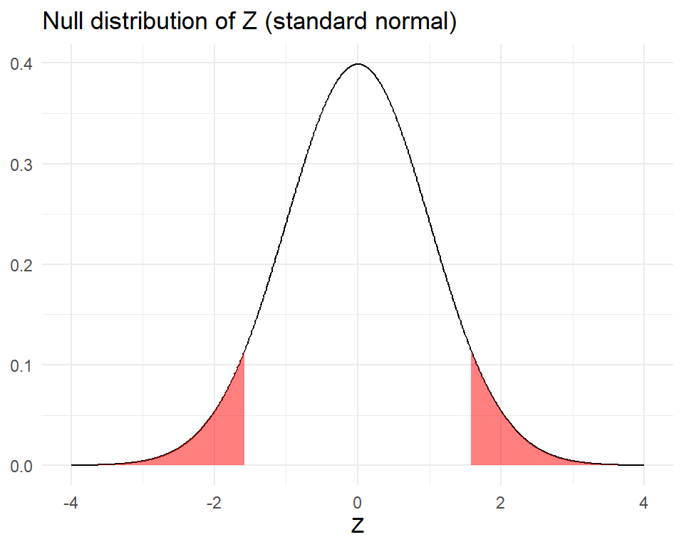
The calculation of the p-value can be done with the $pnorm$ function. The area of both tails combined (2-sided test) is

2*(1 - pnorm(1.578))

## [1] 0.1145656

Note: If we were running a one-sided test, the p-value would have been the area of only one of the tails (that is, we would not have multiplied 1 - pnorm(1.578) by 2).

The p-value can be interpreted as follows:

Under the assumption that the null hypothesis is true (that is, under the assumption that the average 10-mile run time for 2017 was 94.519 minutes), the probability of observing a test statistic $Z$ at least as large (in absolute value) as the one obtained from the sample is 0.114. At a significance level of $\alpha = 0.05,$ this p-value indicates that it’s not highly unlikely to observe a sample average like the one in the current sample, if the null hypothesis was true. Therefore, we do not reject the null hypothesis. We would then say that this sample did not provide evidence that the average run time in the 2017 Cherry Blossom race differed from 94.519 minutes.

Notice that since the sample size was large enough, using a t-distribution would result in a similar p-value and conclusion:

2*(1 - pt(1.578, df = 99))

## [1] 0.1177557

When using a t-distribution, we name the test statistic “T” instead of “Z”, but they are calculated in the same manner.

Using the t.test() function to run a hypothesis test and/or compute a confidence interval for one mean in R.

The sample of 100 runners can be accessed from the openintro website using the following command:

run17samp <- read.csv("https://www.openintro.org/data/csv/run17samp.csv")

To run the hypothesis test, we enter the finishing times (variable clock_sec) as the first input, divided by 60 to convert to minutes, and state the null hypothesis with the input mu = 94.519), as follows:

t.test(run17samp$clock_sec/60, mu = 94.519)

## 
##  One Sample t-test
## 
## data:  run17samp$clock_sec/60
## t = 1.5776, df = 99, p-value = 0.1178
## alternative hypothesis: true mean is not equal to 94.519
## 95 percent confidence interval:
##   93.26973 105.46227
## sample estimates:
## mean of x 
##    99.366

Note that the summary includes the T statistic, the p-value, and a 95% confidence interval for the average finishing time in 2017.

10.3 Confidence interval for $\mu_1 - \mu_2$

Sometimes we may be interested in estimating the difference between the means of two groups, for example, the difference in interest rate between borrowers who have been bankrupt and those who haven’t. We denote the means of the populations for these two groups by $\mu_1$ and $\mu_2$. The best estimate for $\mu_1 - \mu_2$ is $\overline{X}_1 - \overline{X}_2$. However, the Central Limit Theorem gives the approximate sampling distribution of one sample mean, not the difference between two sample means. Thankfully, we can still obtain the sampling distribution of $\overline{X}_1 - \overline{X}_2$ by using the fact that the sum of two normally distributed random variables is also normal.

Denote by $\sigma_1$ and $\sigma_2$ the (population) standard deviations of both groups and by $n_1$ and $n_2$ the sample sizes of the two groups. The fact stated above implies that, for large enough $n_1$ and $n_2$, $\overline{X}_1 - \overline{X}_2$ is approximately normal. Now we just need to find $E(\overline{X}_1 - \overline{X}_2)$ and $Var(\overline{X}_1 - \overline{X}_2)$ in order to find a confidence interval for $\mu_1-\mu_2$:

$$\begin{eqnarray} E(\overline{X}_1 - \overline{X}_2) &=& E(\overline{X}_1) - E(\overline{X}_2) = \mu_1 - \mu_2.\\ Var(\overline{X}_1 - \overline{X}_2) &=& Var(\overline{X}_1) + (-1)^2 Var(\overline{X}_2) \\ &=& \frac{\sigma_1^2}{n_1} + \frac{\sigma_2^2}{n_2}. \end{eqnarray}$$

Here we used the assumption that the data was collected independently for both groups, which implies that $Cov(\overline{X}_1, \overline{X}_2) = 0.$

The calculations above give us the approximate sampling distribution of $\overline{X}_1 - \overline{X}_2$ for large enough $n_1$ and $n_2$ (usually $n_1 \geq 30$ and $n_2 \geq 30$ suffices):

$$\overline{X}_1 - \overline{X}_2 \approx N\left(\mu_1-\mu_2, \sqrt{\frac{\sigma_1^2}{n_1} + \frac{\sigma_2^2}{n_2}}\right).$$

This gives the following result:

Theorem 10.2 (Confidence interval for the difference between two means) Consider iid samples of the same variable for two different groups. Then the endpoints of a $(1-\alpha)$ CI for $\mu_1 - \mu_2$ are given by $$\overline{X}_1 - \overline{X}_2 \pm c\times \sqrt{\frac{S_1^2}{n_1} + \frac{S_2^2}{n_2}}, \quad \mbox{where } c = qnorm(1-\alpha/2).$$ That is, the $(1-\alpha)$ CI is: $$\left[\overline{X}_1 - \overline{X}_2 - c\times \sqrt{\frac{S_1^2}{n_1} + \frac{S_2^2}{n_2}}, \overline{X}_1 + \overline{X}_2 + c\times \sqrt{\frac{S_1^2}{n_1} + \frac{S_2^2}{n_2}}\right], \quad \mbox{where } c = qnorm(1-\alpha/2).$$

If $n_1$ or $n_2$ are not large enough and if the data for both groups could come from a normal distribution (no extreme skew is present), the t distribution should be used to find the critical value. That is, $$c = qt(1-\alpha/2, df),$$ where

$$\begin{equation} df = \frac{\left(\frac{S_1^2}{n_1}+\frac{S_2^2}{n_2}\right)^2}{\frac{\left(\frac{S_1^2}{n_1}\right)^2}{n_1-1}+\frac{\left(\frac{S_2^2}{n_2}\right)^2}{n_2-1}} \approx min(n_1-1, n_2-1). \tag{10.1} \end{equation}$$

One can also use the t distribution to calculate $c$ even when $n_1$ and $n_2$ are large enough. This is because the t distribution approaches the standard normal as the degrees of freedom increase.

Example 10.3 Suppose that we want to estimate the difference in interest rate between borrowers (from peer-to-peer lending) who have been bankrupt and those who haven’t. We will use the loans dataset to provide a 95% CI for this difference. First, we need to create a variable that indicates whether someone has any history of bankruptcy.

loans <- loans |>
  mutate(bankruptcy = if_else(public_record_bankrupt == 0, "no", "yes"))

The function if_else assigns “no” to the variable bankruptcy if the borrower’s public record shows no bankruptcies, and it assigns “yes” otherwise. Now we can find $\overline{X}_1$, $\overline{X}_2$, $S_1$, $S_2$, $n_1$, and $n_2$:

loans |>
  group_by(bankruptcy) |>
  summarize(xbar = mean(interest_rate, na.rm = T),
            S = sd(interest_rate, na.rm = T),
            n = n())

## # A tibble: 2 × 4
##   bankruptcy  xbar     S     n
##   <chr>      <dbl> <dbl> <int>
## 1 no          12.3  5.02  8785
## 2 yes         13.1  4.83  1215

That is, the interest_rate sample average, standard deviation, and size for the non-bankrupt group are $\overline{X}_1 = 12.33$%, $S_1 = 5.018$%, and $n_1 = 8785$, while for the bankrupt group these quantities are $\overline{X}_2 = 13.07$%, $S_2 = 4.830$%, and $n_2 = 1215$. The critical value for a 95% CI is qnorm(1 - 0.05/2) = 1.96. Now we are ready to calculate the confidence interval:

$$\begin{eqnarray} \overline{X}_1 - \overline{X}_2 \pm c\times \sqrt{\frac{S_1^2}{n_1} + \frac{S_2^2}{n_2}} &=& 12.338 - 13.075 \pm 1.96\sqrt{\frac{5.018^2}{8785} + \frac{4.830^2}{1215}} \\ &=& -0.737 \pm 0.291 = [-1.028, -0.445] \end{eqnarray}$$

This means that we are 95% confident that the difference between the interest rates for those who have been bankrupt and those who haven’t is between -1.028% and -0.445%. Since 0 is not included in this interval, then this is statistical evidence that the average interest rate for the two groups is not the same. We would then say that there is a statistically significant difference between the two groups. More specifically, the data indicates that those with a history of bankrupcy tend to have a higher interest rate.

Let’s re-calculate the critical value $c$ from example 10.3 using the t distribution:

S1 <- 5.018019
S2 <- 4.829929
n1 <- 8785
n2 <- 1215
df <- (S1^2/n1 + S2^2/n2)^2/((S1^2/n1)^2/(n1 - 1) + (S2^2/n2)^2/(n2 - 1))
qt(1 - 0.05/2, df)

## [1] 1.961449

In this case, because $n_1$ and $n_2$ are so large, we get the same critical value using qnorm or qt.

10.4 Hypothesis testing for $\mu_1 - \mu_2$

In this section, we describe the procedure to test hypotheses of the type:

$H_0:$ $\mu_1 - \mu_2 = 0$

$H_a:$ $\mu_1 - \mu_2 \neq 0$

That is, hypotheses for the difference between two population means. Again, we can have one-sided hypotheses instead of two-sided ones. The value 0 can be replaced with a non-zero one, but the most common choice is 0 because it is more common to be interested in whether two population means are equal.

To perform a hypothesis test for $\mu_1 - \mu_2$ using the CLT, we calculate $$Z = \frac{\overline{X}_1-\overline{X}_2}{\sqrt{\frac{S_1^2}{n_1} + \frac{S_2^2}{n_2}}}.$$

The denominator is the approximate standard deviation of $\overline{X}_1 - \overline{X}_2.$ For large enough $n_1$ and $n_2$ (usually $n_1, n_2 \geq 30$ suffices), the null distribution of $Z$ is approximately a standard normal distribution. The p-value is then the probability that, under the null hypothesis, one would observe a test statistic $Z$ at least as large (in absolute value) as the one obtained from the data. If one of $n_1$ or $n_2$ is not as large (usually between 10 and 30), the t-distribution may be used instead of the normal (with the degrees of freedom given by equation (10.1)), if the population distribution of both groups can be reasonably considered to be normal.

Example 10.4 Prices of diamonds are determined by what is known as the 4 Cs: cut, clarity, color, and carat weight. The prices of diamonds go up as the carat weight increases, but the increase is not smooth. For example, the difference between the size of a 0.99 carat diamond and a 1 carat diamond is undetectable to the naked human eye, but the price of a 1 carat diamond tends to be much higher than the price of a 0.99 diamond. The dataset diamonds from the ggplot2 package has a large sample of diamonds that we can use to compare 0.99 and 1 carat diamonds. In order to be able to compare equivalent units, we divide the price of each diamond by its weight in carats. In that way, we can compare the average price per carat for 0.99 and 1 carat diamonds. The sample statistics and a side-by-side boxplot are shown below.

library(tidyverse)
diamonds2 <- diamonds |> 
  mutate(price_per_carat = price/carat) |> 
  filter(carat == 1 | carat == .99)
summaries <- diamonds2 |> 
  group_by(carat) |> 
  summarize(M = mean(price_per_carat, na.rm = T),
            SD = sd(price_per_carat, na.rm = T), 
            n = n())
summaries |> knitr::kable(format = "html")

carat	M	SD	n
0.99	4450.681	1332.311	23
1.00	5241.590	1603.939	1558

ggplot(diamonds2, aes(y = price_per_carat, x = factor(carat))) +
  geom_boxplot(alpha = 0.5) +
  labs(y = "Price per carat", x = "Weight (in carat)")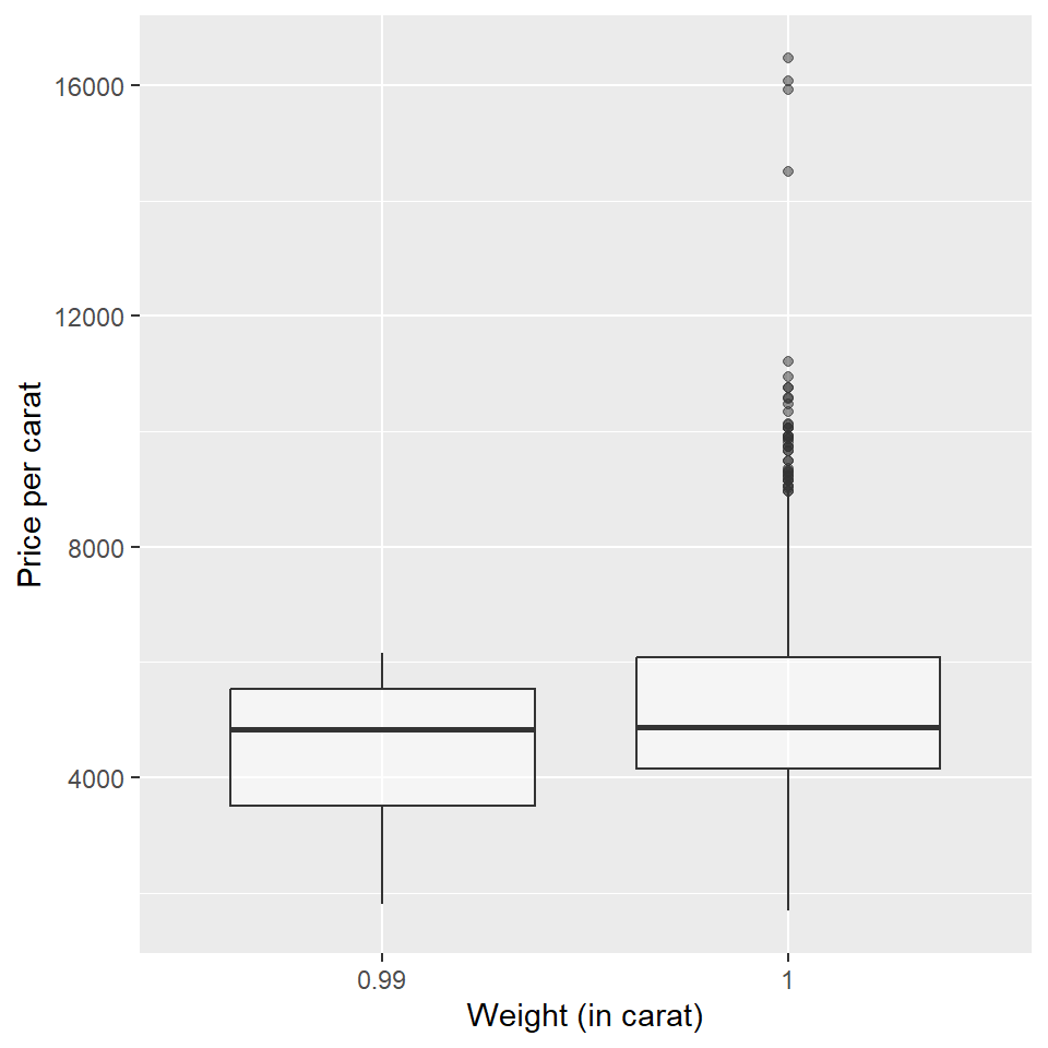

Next, we run a hypothesis test to evaluate if there is a difference between the price (per carat) of 0.99 and 1 carat diamonds. The hypotheses we are testing are:

$H_0$: $\mu_1 - \mu_2 = 0$

$H_a$: $\mu_1 - \mu_2 \neq 0,$

where $\mu_1$ is the mean price per carat of 0.99 carat diamonds and $\mu_2$ is the mean price per carat of 1 carat diamonds.

The test statistic is

$$Z = \frac{4450.681 - 5241.590}{\sqrt{\frac{1332.311^2}{23}+\frac{1603.939^2}{1558}}} = -2.817$$

If both $n_1$ and $n_2$ are large enough, under $H_0$, $Z \approx N(0,1)$ and the p-value can be calculated as

2*pnorm(-2.817)

## [1] 0.004847453

or

2*(1 - pnorm(2.817))

## [1] 0.004847453

The small p-value supports the alternative hypothesis. That is, the difference between the average price per carat of 0.99 and 1 carat diamonds is statistically significant.

If $n_1$ or $n_2$ are not large enough but their data could come from a normal distribution (no extreme skew is present), the t distribution should be used to find the p-value. That is, $$\mbox{p-value} = 2\times pt(-|T|, df) = 2\times (1-pt(|T|,df)),$$ where $$df = \frac{\left(\frac{S_1^2}{n_1}+\frac{S_2^2}{n_2}\right)^2}{\frac{\left(\frac{S_1^2}{n_1}\right)^2}{n_1-1}+\frac{\left(\frac{S_2^2}{n_2}\right)^2}{n_2-1}}.$$

In the previous example, if using the t distribution (note that $n_1$ is small), $df=22.951$ and the p-value would be 0.0098, as shown in the calculations below.

S1 <- 1332.311
S2 <- 1603.939
n1 <- 23
n2 <- 1558
df <- (S1^2/n1 + S2^2/n2)^2/((S1^2/n1)^2/(n1 - 1) + (S2^2/n2)^2/(n2 - 1)); df

## [1] 22.95133

pvalue <- 2*pt(-2.817, df); pvalue

## [1] 0.009792158

Using the function t.test() to run a hypothesis test and/or find a confidence interval for the difference between two means. The input is a formula numerical_variable ~ grouping_variable and the data. For the diamonds example:

t.test(price_per_carat ~ carat, data = diamonds2)

## 
##  Welch Two Sample t-test
## 
## data:  price_per_carat by carat
## t = -2.817, df = 22.951, p-value = 0.009792
## alternative hypothesis: true difference in means between group 0.99 and group 1 is not equal to 0
## 95 percent confidence interval:
##  -1371.7782  -210.0401
## sample estimates:
## mean in group 0.99    mean in group 1 
##           4450.681           5241.590

Note that the summary includes the T statistic, the p-value, and a 95% confidence interval for the difference in prices.

10.5 A few remarks about hypothesis tests

10.5.1 Hypothesis tests for other parameters

As you may have noticed, hypothesis tests (HTs) are built by first stating two complementary hypotheses (null and alternative). We then calculate the probability that one would observe a sample at least as favorable to the alternative hypothesis as the current sample, if the null hypothesis was true. This sequence of steps can be taken for conducting tests about several population parameters (for example, means, proportions, standard deviations, slopes of regression lines, etc). Notice that the key to the development of such tests was gaining an understanding of the null distribution of an estimator, that is, the sampling distribution of an estimator under the assumption that $H_0$ was true.

10.5.2 Statistical significance versus practical significance

As the sample size becomes larger, point estimates become more precise and any real differences in the sample estimate and null value become easier to detect and recognize. Even a very small difference would likely be detected if we took a large enough sample. In such cases, we still say the difference is statistically significant, but it is not practically significant. For example, an online experiment might identify that placing additional ads on a movie review website statistically significantly increases viewership of a TV show by 0.001%, but this increase might not have any practical value. Therefore, it is important to interpret the practical implications of a result and not simply rely on statistical significance as the “final” result.

---

27. The proof of this result is beyond the scope of this course.↩︎