5 Probability

The theoretical foundation of statistics is based on probability, and while probability is not required for applying the techniques learned in this course, it helps you gain a deeper understanding of the methods and set a better foundation for using statistics.

We use probability to build tools to describe and understand apparent randomness. We often frame probability in terms of a random experiment giving rise to an outcome. For example, rolling a die and flipping a coin can be considered random experiments and that give rise to an outcome.

Roll a die \(\rightarrow\) 1, 2, 3, 4, 5, or 6

Flip a coin \(\rightarrow\) H or T

There are two commonly used interpretations of probability in statistics: frequentist and bayesian. In the frequentist interpretation, which is the more traditional one, the probability of an outcome is the proportion of times the outcome would occur if we observed the random experiment an infinite number of times. In the bayesian interpretation, probability is interpreted as a reasonable expectation based on knowledge or a personal belief. In this course, we use the frequentist interpretation.

For example, in the frequentist interpretation, the probability of getting heads in a coin flip is the proportion of heads one would get when flipping a coin an “infinite” amount of times. In the bayesian interpretation, one would use some knowledge or personal belief, for example, the belief that the coin is unbiased, to say that the probability of getting heads is 0.5. This prior probability can then be updated to a posterior probability any time we gain new information (data) regarding the fairness of the coin.

The following code is a simulation of 1000 coin flips in R.

n <- 1000 # number of times you flip a coin
S <- c("H", "T") # possible outcomes of each coin toss: H or T
flips <- sample(S, n, replace = TRUE) # draw from S n times, with replacement
freq <- table(flips)/n; freq # print relative frequencies

## flips
##     H     T 
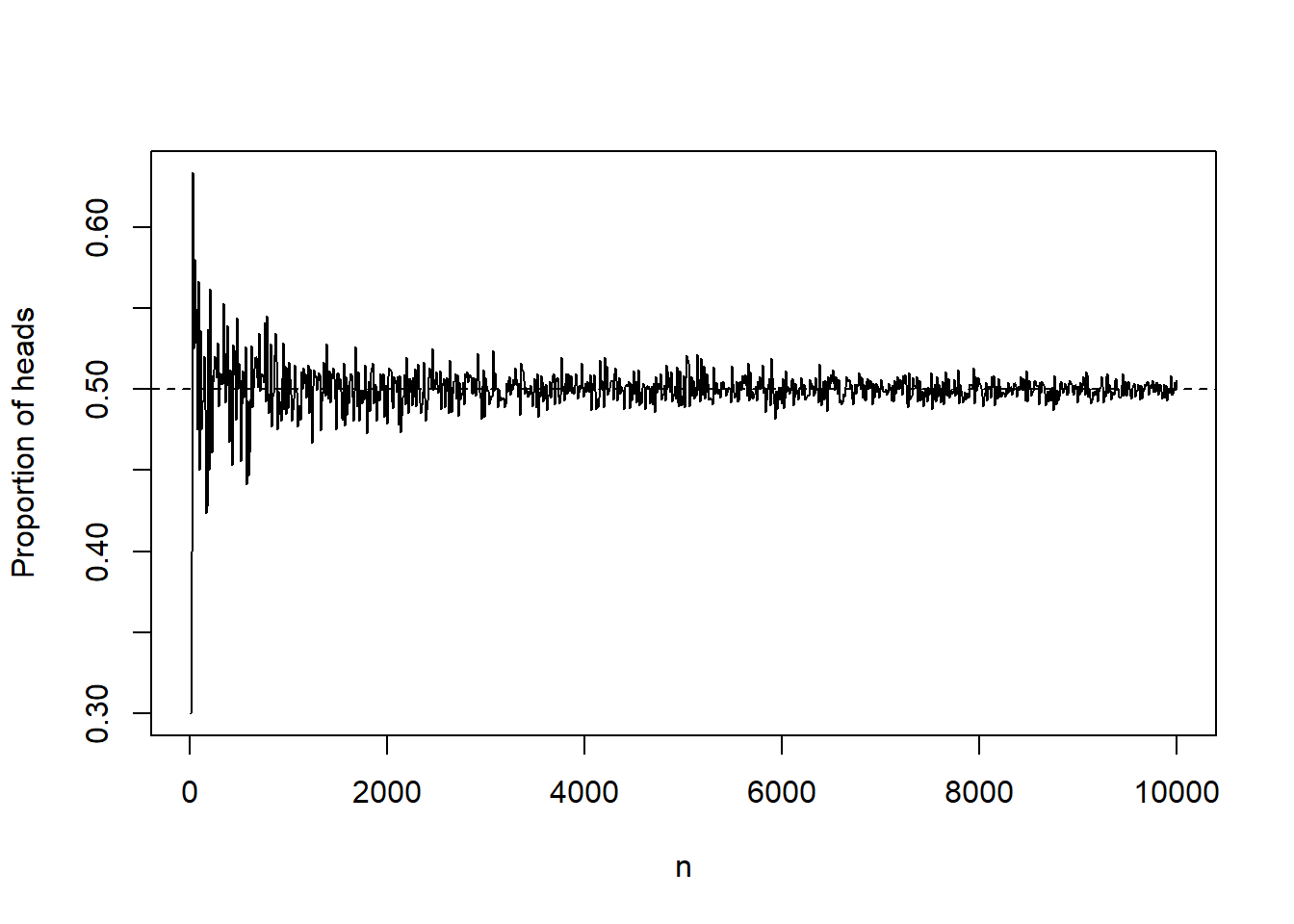
## 0.477 0.523

In this simulation, heads occurred 47.7% of the time. As we increase \(n\), the proportion of heads should get closer and closer to 50% (try for yourself!)

5.1 Definitions, laws, and examples

Theorem 5.1 (Law of Large Numbers) As more trials of the same random experiment are performed, the proportion of occurrences with a particular outcome converges to the probability of that outcome.

As an illustration of the Law of Large Numbers (LLN), running the coin flip code above for several values of \(n\), gives the following proportions of heads:

Definition 5.1 (Sample space) The sample space (or outcome space) of a random experiment is the set of all possible outcomes of the experiment. It is denoted by \(\Omega\).

For example, if the random experiment is to flip two coins, then \(\Omega = \{HH, HT, TH, TT\}\).

Definition 5.2 (Random variable) A random variable is a function that assigns a real number to each outcome in a sample space.

For example, when flipping two coins, the number of heads obtained, let’s call it \(X\), is a random variable. More specifically, \(X(HH) = 2\), \(X(HT) = 1\), \(X(TH) = 1\), and \(X(TT) = 0\).

Estimates made from a sample about a population are also random variables. For example, the sample average, \(\overline{X}\), and the LS regression slope, \(\hat{b}\), are random variables (is it clear why?).

Definition 5.3 (Event) An event is a subset of the sample space.

For example, “at least one head” is an event of two coin flips. This event is the set \(\{HH, HT, TH\}\), which is a subset of \(\Omega = \{HH, HT, TH, TT\}\).

Definition 5.4 (Operations with events) The following are definitions of operations with events.

The union of two events A and B, denoted \(A\cup B\), is the subset of the sample space in which \(A\) or \(B\) happens. Here the word “or” is inclusive, meaning that \(A\) and \(B\) can possibly happen simultaneously.
The intersection of two events A and B, denoted \(A\cap B\), is the subset of the sample space in which \(A\) and \(B\) happen simultaneously.
The complement of an event A, denoted \(A^c\), is the subset of the sample space in which \(A\) does not occur.
Two events A and B are said to be disjoint or mutually exclusive if they cannot happen simultaneously. That is, when \(A\cap B\) is empty, denoted \(A\cap B = \emptyset\).

Addition rule of disjoint events: If \(A_1\) and \(A_2\) represent two disjoint events, then the probability that one of them occurs is given by \[P(A_1 \cup A_2) = P(A_1) + P(A_2).\] If there are many disjoint events \(A_1, \dots, A_k,\) then the probability that one of these events will occur is \[P(A_1 \cup A_2 \cup \cdots \cup A_k) = P(A_1) + P(A_2) + \cdots + P(A_k).\]

For example, when rolling a die, the events 1 and 2 are disjoint, and we compute the probability that one of these events will occur by adding their separate probabilities: \(P(1 \cup 2) = P(1) + P(2) = 1/6 + 1/6 = 1/3.\) Notice that \(P(1\cup 2\cup 3\cup 4 \cup 5 \cup 6) = 1/6 + 1/6+1/6 + 1/6+1/6 + 1/6 = 1,\) that is, the probability of the sample space is 1.

Another consequence of the addition rule for disjoint events is that \(P(A^c) = 1 - P(A),\) for any event \(A\). This is because \(A\cup A^c = \Omega\) and therefore, \(1 = P(A\cup A^c) = P(A) +P(A^c)\), which implies that \(P(A^c) = 1-P(A)\).

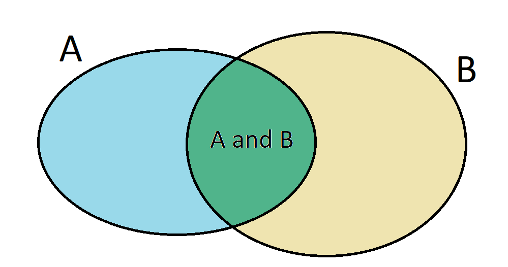
General Addition Rule: If \(A\) and \(B\) are any two events, disjoint or not, then the probability that at least one of them will occur is \[P(A\cup B) = P(A) + P(B) - P(A\cap B).\] A Venn diagram can help visualize why one needs to subtract \(P(A\cap B)\) in the General Addition Rule: if we simply add \(P(A)\) and \(P(B)\), we will include their intersection twice, so we must subtract it once.

Example 5.1 Let’s consider calculations for two events that are not disjoint in the context of a regular deck of 52 cards. Let \(A\) represent the event that a randomly selected card is a diamond and \(B\) represent the event that it is a face card. How do we compute \(P(A \cup B)\)? Events \(A\) and \(B\) are not disjoint (the cards \(J\diamondsuit\), \(Q\diamondsuit\), and \(K\diamondsuit\) fall into both categories) so we cannot use the addition rule for disjoint events. Instead we use the General Addition Rule: \[\begin{eqnarray} P(A \cup B) &=& P(\diamondsuit) + P(\mbox{face card}) - P(\diamondsuit \cap \mbox{face card}) \\ &=& 13/52 + 12/52 - 3/52 = 22/52 = 0.423. \end{eqnarray}\]

5.2 Independence

Two experiments/processes are independent if knowing the outcome of one provides no useful information about the outcome of the other. For instance, flipping a coin and rolling a die are two independent processes (knowing the coin was heads does not help determine the outcome of a die roll.) On the other hand, stock prices usually move up or down together, so they are not independent.

Example 5.2 Consider the random experiment of rolling two dice, a red and a white one. We want to determine the probability that both will be 1. If the outcome of the red die is a 1, it provides no information about the outcome of the white die. More specificlly, the probability of getting a 1 in the red die is 1/6 and the probability of getting a 1 in the white die is 1/6. Because the rolls are independent, the probabilities of the corresponding outcomes can be multiplied to get the final answer: \(\frac{1}{6}\times\frac{1}{6} = 1/36.\) This can be generalized to many independent processes.

Multiplication rule for independent processes: If \(A\) and \(B\) represent events from two different and independent processes, then the probability that both \(A\) and \(B\) occur can be calculated as the product of their separate probabilities: \[P(A \cap B) = P(A) \times P(B).\] Similarly, if there are \(k\) events \(A_1, \dots, A_k\) from \(k\) independent processes, then the probability they all occur is \[P(A_1) \times P(A_2) \times \cdots \times P(A_k).\]

Example 5.3 About 9% of people are left-handed, and about 18% of people have an attached earlobe. Suppose the variables handedness and earlobe are independent, i.e. knowing someone’s handedness provides no useful information about their earlobes and vice-versa. We can then compute whether a randomly selected person is right-handed (RH) and has an attached earlobe (AE) using the multiplication rule: \[P(\mbox{RH and AE}) = P(\mbox{RH}) \times P(\mbox{AE}) = (1-0.09)\times 0.18 = 0.1638.\]

Now suppose that 5 people are selected at random.

What is the probability that all are right-handed?
What is the probability that not all of the people are right-handed?
What is the probability that the first person has a detached earlobe and is right-handed?
What is the probability that the first two people have a detached earlobe and right-handed?

Answers:

The abbreviations RH and LH are used for right-handed and left-handed, respectively. Notice that the probability of being right-randed is \(1-P(\mbox{LH}) = 1-0.09 = 0.91\), because RH is the complement of LH. Since each are independent, we apply the Multiplication Rule for independent processes: \[\begin{eqnarray} P(\mbox{all five are RH}) &=& P(\mbox{first is RH, second is RH, ..., fifth is RH})\\ &=& P(\mbox{first is RH}) \times P(\mbox{second is RH}) \times \cdots \times P(\mbox{fifth is RH})\\ &=& 0.91 \times 0.91 \times 0.91 \times 0.91 \times 0.91 = 0.624. \end{eqnarray}\]
Use the complement of P(all five are RH), to answer this question: \[P(\mbox{not all RH}) = 1 - P(\mbox{all five are RH}) = 1- 0.624 = 0.376.\]
Here we use the abbreviations DE and AE for “detached earlobe” and “attached earlobe”, respectively. \[P(\mbox{DE and RH}) = P(\mbox{DE})\times P(\mbox{RH}) = (1-0.18)\times 0.91 = 0.7642.\]
Using part (c) and the multiplication rule for independent events: \[\begin{eqnarray} P(\mbox{first two are DE and RH}) &=& P(\mbox{first is DE and RH})\times P(\mbox{second is DE and RH})\\ &=& 0.7642\times 0.7642 = 0.584. \end{eqnarray}\]

5.3 Conditional probability

5.3.1 Definitions

We motivate the definition of conditional probability with the following example.

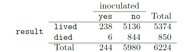
Example 5.4 The smallpox dataset (openintro package) provides a sample of 6,224 individuals from the year 1721 who were exposed to smallpox in Boston. Doctors at the time believed that inoculation, which involves exposing a person to the disease in a controlled form, could reduce the likelihood of death.

Each case represents one person with two variables: inoculated and result. The variable inoculated takes two levels: yes or no, indicating whether the person was inoculated or not. The variable result has outcomes lived or died. These data are summarized below in a contingency table (left) and then dividing each count by the table total, 6224 (right).

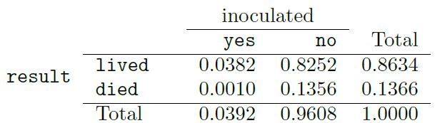
The probabilities in the middle of the table on the right (0.0382, 0.8252, 0.0010, and 0.1356) are called joint probabilities since they compute the probability of the joint outcome of two variables. For instance,

\(P(\{\)result = died\(\} \cap \{\)inoculated = yes}\() = \frac{6}{6224} = 0.001.\)

The row and column totals (0.8634, 0.1366, 0.0392, 0.9608) are called marginal probabilities, since they are typically reported on the margins of the table. These probabilities are based on a single variable without regard to any other variables. For instance, the probability of dying from smallpox is a marginal probability:

\(P(\)result = died\() = \frac{850}{6224} = 0.1366.\)

However, for someone who was inoculated, does this probability change? In other words, can we take into account knowledge we have about someone being inoculated to compute the probability of dying from smallpox?

For example, the probability that a randomly selected person died from smallpox given that the person was inoculated is:

\(P(\{\)result = died\(\}\) given \(\{\)inoculated = yes\(\}) = \frac{6}{244} = 0.0246\).

We call this a conditional probability because we computed the probability under a condition: the person was unoculated.

There are two parts to a conditional probability, the outcome of interest and the condition. It is useful to think of the condition as information we know to be true, and this information usually can be described as a known outcome or event.

Definition 5.5 The conditional probability of outcome \(A\) given condition \(B\) is computed as the following: \[P(A | B) = \frac{P(A \cap B)}{P(B)} = \frac{P(A \mbox{ and } B)}{P(B)} = \frac{P(A, B)}{P(B)}.\]

Here the vertical bar replaces the word “given”.

Back to the previous example, using this new notation, the probability a randomly selected person who was inoculated died from smallpox is:

\[\begin{eqnarray} P(\mbox{result = died | inoculated = yes}) &=& \frac{P(\mbox{result = died, inoculated = yes})}{P(\mbox{inoculated = yes})} \\ &=& \frac{6/6224}{244/6224} = \frac{6}{244} = 0.0246. \end{eqnarray}\]

The probability a randomly selected person who was not inoculated died from smallpox is:

\[\begin{eqnarray} P(\mbox{result = died | inoculated = no}) &=& \frac{P(\mbox{result = died, inoculated = no})}{P(\mbox{inoculated = no})} \\ &=& \frac{844/6224}{5980/6224} = \frac{844}{5980} = 0.1411. \end{eqnarray}\]

That is, the death rate for individuals who were inoculated is about 2.5% (1 in 40) while the death rate is about 14% (1 in 7) for those who were not inoculated.

5.3.2 General multiplication rule

In section 5.2, we introduced the multiplication rule for independent processes. Here we provide the general multiplication rule for events that might not be independent.

General multiplication rule:

If \(A\) and \(B\) represent outcomes from two (not necessarily independent) processes, then the probability that both \(A\) and \(B\) occur can be calculated as: \[P(A \cap B) = P(A | B) \times P(B).\]

It is useful to think of A as the outcome of interest and B as the condition.

Example 5.5 Consider the smallpox data set. Suppose we are given only two pieces of information: 96.08% of residents were not inoculated, and 85.88% of the residents who were not inoculated ended up surviving. How could we compute the probability that a resident was not inoculated and lived?

Using the general multiplication rule: \[\begin{eqnarray} P(\mbox{result = lived, inoculated = no}) &=& P(\mbox{result = lived | inoculated = no})\times P(\mbox{inoculated = no})\\ &=& 0.8588\times 0.9608 = 0.8251. \end{eqnarray}\]

Tree diagrams:

Tree diagrams are a tool to organize outcomes and probabilities around the structure of the data. They are most useful when two or more processes occur in a sequence and each process is conditioned on its predecessors. The smallpox data fit this description. We see the population as split by inoculation: yes and no. Following this split, survival rates were observed for each group. This structure is reflected in the tree diagram below.

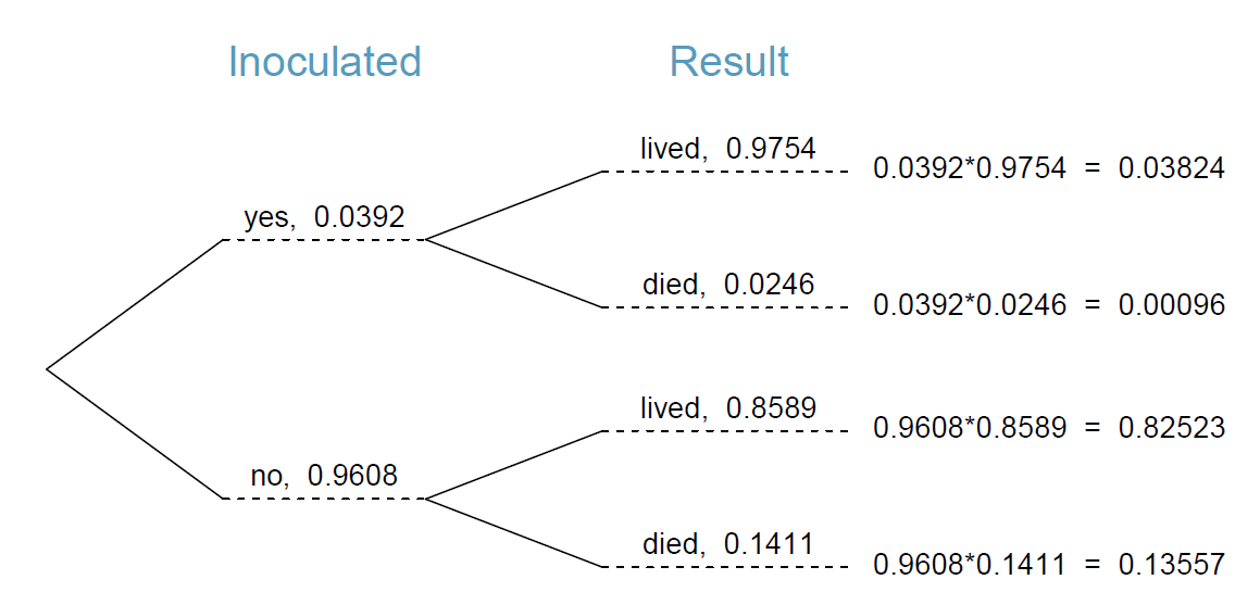
Tree diagrams are annotated with marginal and conditional probabilities, as shown above. This tree diagram splits the smallpox data by inoculation into the yes and no groups with respective marginal probabilities 0.0392 and 0.9608. The secondary branches are conditioned on the first, so we assign conditional probabilities to these branches. For example, the top branch is the probability that result = lived conditioned on the information that inoculated = yes. We may (and usually do) construct joint probabilities at the end of each branch in our tree by multiplying the numbers we come across as we move from left to right. These joint probabilities are computed using the general multiplication rule.

5.3.3 Bayes Theorem

In many instances, we are given a conditional probability of the form P(A | B) but we would really like to know the inverted conditional probability P(B | A). Tree diagrams can be used to find the second conditional probability when given the first. However, sometimes it is not possible to draw the scenario in a tree diagram. In these cases, we can apply a very useful and general formula: Bayes’ Theorem. We first take a critical look at an example of inverting conditional probabilities where we still apply a tree diagram.

Example 5.6 In Canada, about 0.35% of women over 40 will develop breast cancer in any given year. A common screening test for cancer is the mammogram, but this test is not perfect. In about 11% of patients with breast cancer, the test gives a false negative: it indicates a woman does not have breast cancer when she does have breast cancer. Similarly, the test gives a false positive in 7% of patients who do not have breast cancer: it indicates these patients have breast cancer when they actually do not. If we tested a random woman over 40 for breast cancer using a mammogram and the test came back positive (that is, the test suggested the patient has cancer) what is the probability that the patient actually has breast cancer?

Notice that we are given sufficient information to quickly compute the probability of testing positive if a woman has breast cancer (1 - 0.11 = 0.89). However, we seek the inverted probability of cancer given a positive test result. (Watch out for the non-intuitive medical language: a positive test result suggests the possible presence of cancer in a mammogram screening.) This inverted probability may be broken into two pieces: \(P(BC | +) = \frac{P(BC \cap +)}{P(+)},\) where “BC” is an abbreviation for the patient having breast cancer and “+” means the mammogram screening was positive. We can construct a tree diagram for these probabilities:

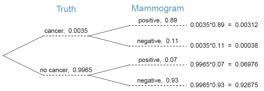
The probability the patient has breast cancer and the mammogram is positive is \(P(+ | BC)P(BC) = 0.89 \times 0.0035 = 0.00312.\) The probability of a positive test result is the sum of two scenarios: \(P(+ \cap BC) + P(+ \cap BC^c) = 0.0035 \times 0.89 + 0.9965 \times 0.07 = 0.07288.\)

Then if the mammogram screening is positive for a patient, the probability the patient has breast cancer is \[P(BC|+) = \frac{P(BC|+)}{P(+)} = \frac{0.00312}{0.07288} = 0.0428.\]

That is, even if a patient has a positive mammogram screening, there is still only a 4% chance that she has breast cancer. This example highlights why doctors often run more tests regardless of a first positive test result. When a medical condition is rare, a single positive test isn’t generally definitive.

Through inspecting the calculations above, we can see that \[P(BC | +) = \frac{P(+ | BC)P(BC)}{P(+ | BC)P(BC) + P(+ | BC^c)P(BC^c)}.\]

This formula is known as Bayes’ theorem, which can be stated in a more general form as follows.

Theorem 5.2 Bayes’ theorem. Consider outcomes \(A_1, A_2, A_3, \dots, A_k\) for variable 1 and outcome \(B\) for variable 2. Then \[P(A_1 | B) = \frac{P(B | A_1)P(A_1)}{P(B | A_1)P(A_1) + P(B | A_2)P(A_2) + \cdots + P(B|A_k)P(A_k)}.\]

Bayes’ Theorem is a generalization of what we have done using tree diagrams. The numerator identifies the probability of getting both \(A_1\) and \(B.\) The denominator is the marginal probability of getting \(B.\) This bottom component of the fraction appears long and complicated since we have to add up probabilities from all of the different ways to get \(B.\) We completed this step when using tree diagrams. However, we usually did it in a separate step so it didn’t seem as complex.

The strategy of updating probabilities using Bayes’ Theorem is the foundation of an entire area of statistics called Bayesian statistics.