1 Data Basics
1.1 R and RStudio essentials
Since we will use R and RStudio to illustrate concepts and give examples throughout these notes, it makes sense to begin by introducing these platforms.
1.1.1 The basics
R is a programming language and environment for statistical computing and graphics1.
RStudio is an integrated development environment (IDE) for R , which includes a console, syntax-highlighting editor that supports direct code execution, as well as tools for plotting, history, debugging and workspace management2. Both are free and open source3. RStudio is the interface through which we will use R.
Posit Cloud is a hosted version of RStudio on the cloud.
To navigate through this course, you will need to either
Download and install R and RStudio (instructions here), or
Join the MA217 workspace on Posit Cloud (instructions here).
Once you launch RStudio ![]() . You should see an interface similar to this one:
. You should see an interface similar to this one:
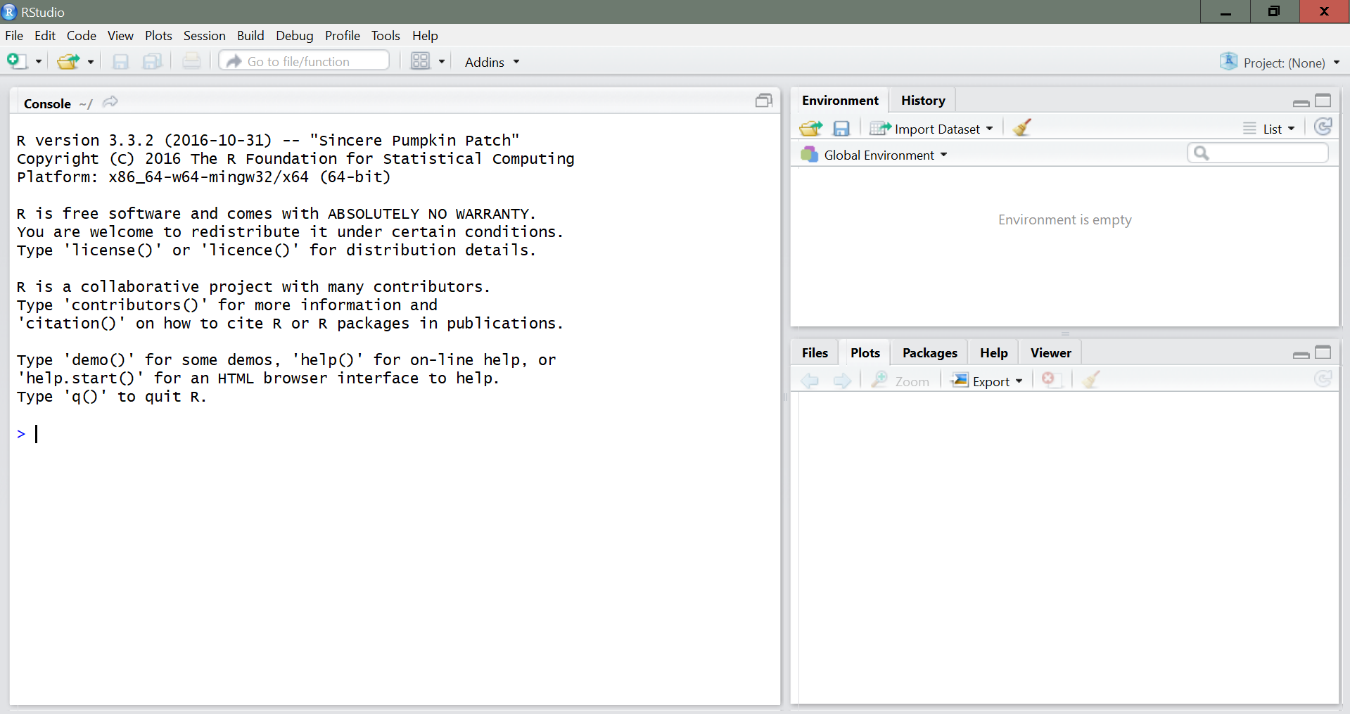
The panel in the upper right contains your workspace as well as a history of the commands that you have previously entered. Any plots that you generate will show up in the panel in the lower right corner.
The panel on the left is where the action happens. It’s called the console. Every time you launch RStudio, it will have the same text at the top of the console telling you the version of R that you’re running. Below that information is the prompt, indicated by the > symbol. As its name suggests, this prompt is a request for a command. Initially, interacting with R is all about typing commands and interpreting the output. These commands and their syntax have evolved over decades (literally) and now provide what many users feel is a fairly natural way to access data and organize, describe, and invoke statistical computations.
Performing simple calculations in R is a good way to begin
learning its features. Commands entered in the console are immediately executed by R. Most simple calculations will work just like you would expect from a typical calculator. For example, typing 3+5 in the console will return 8 (try it for yourself).
## [1] 8Other examples:
## [1] 15## [1] 9This last example demonstrates how functions are called within R as well as the use of comments. Comments are prefaced with the # character. You can also save values to named variables for later reuse.
## [1] 3The assignment operator <- assigns 1 + 2 to a variable named simple_sum4. We read that code as “simple_sum gets 1 + 2”. Note that the value of simple_sum is not printed, it’s just stored. If you want to view the value, type simple_sum in the console.
You will make lots of assignments, so you can save time with RStudio’s keyboard shortcut: Alt - (the minus sign). Notice that RStudio automatically surrounds <- with spaces, which is a good code formatting practice.
Once variables are defined, they can be referenced in other operations and functions.
## [1] 1.5## [1] 1.098612Note that R is case sensitive, so simple_Sum would be a different variable than simple_sum.
We can create a set of values, which we’ll refer to as a vector, using the concatenate (combine) function c(), such as:
a <- c(-1, 1, 0, 5, 2, -3) # creates a vector called 'a' with six values in it
a[2] # displays the second component of a
## [1] 1## [1] -1 1 0 5 2 -3Basic arithmetic can also be carried out on vectors. These operations are carried out componentwise. For example, we could multiply each component of a by itself via
## [1] 1 1 0 25 4 9or multiply each element of a by 2 as in
## [1] -2 2 0 10 4 -6R also operates on logical quantities TRUE (or T for true) and FALSE (or F for false). Logical values are generated by conditions that are either true or false. For
example,
## [1] FALSE TRUE TRUE FALSE FALSEcompares each element of the vector a with 0, returning TRUE when it is greater than 0 and FALSE otherwise. The following logical operators can be used: <, <=, >=, >, == (for equality), != (for “not equal”), as well as & (for intersection), | (for union) and ! (for negation).
Sometimes we may have variables that take character values. While it is always possible to code these values as numbers, there is no need to do this, as R can also handle character-valued variables. For example, the commands
## [1] "MA117" "MA217" "MA237" "MA417"creates a character vector named stats_courses, containing four values, and then we print out this vector. Note that we included the character values in quotes when doing the assignment.
Sometimes data values are missing and so are listed as NA (not available). Operations on missing values create missing values. Also, an impossible operation, such as 0/0, produces NaN (not a number), and an operation such as 3/0 produces Inf.
1.1.2 Calling functions
R has a large collection of built-in functions. For example, to find the mean of a set of values, we use the function mean():
## [1] 3.5If missing values are present, we can ask R to remove them prior to computing the mean by adding the argument na.rm = TRUE to the call of the function:
## [1] 3.333333To learn about all possible arguments in a function type ?function_name in your console. For the function mean, we type ?mean. This shows that the first argument of mean() is x, the second is trim, and the third is na.rm. When we don’t specify a certain argument, R takes the default value for that argument (if there’s one). The default value for trim is trim = 0 (that is, no trimming).
We can omit the argument’s name in a function call if we provide the arguments in order. For example, the call above could also be made as:
## [1] 3.333333R took the first argument as x. We could not omit na.rm = because R would have taken the second input as trim =. Try typing mean(c(2, 3, NA, 5), TRUE) in your console. You will get the following an error message:

Various objects can be created during an R session. To see those created so far in your session, use the command ls(). You can remove any objects in your workspace using the command rm(). For example, rm(stats_courses) removes the vector stats_courses.
1.1.3 The pipe operator
Combining multiple functions in R can get cumbersome, and we’ll do so with the pipe: |>. The pipe takes the object on its left and passes it along to the function on its right so that x |> f() is equivalent to f(x), and x |> f(y) is equivalent to f(x, y). Going further, x |> f(y) |> g(z) is equivalent to g(f(x, y), z). The easiest way to pronounce the pipe is “then”. For example, the command below can be read as: Take the vector c(1, 2, 3, 4, 5) then find its mean then compute the log.
## [1] 1.098612The command above are equivalent to
## [1] 1.098612In the latest versions of R, the native pipe operator |> is now the default for chaining functions, replacing the previously common tidyverse pipe (%>%) that was loaded with the dplyr package. You’ll still often see R code using %>% in older scripts or searches online, but we’ll use |> in this course.
1.1.4 Working with R Script Files
As an alternative to typing commands directly into the console, R commands can be stored in a file, called an R script, which facilitates executing some or all of the commands at any time. To create a file, select File, then New File, then R Script from the RStudio menu. A file editor tab will open in the Source panel. R code can be entered there, and buttons and menu items are provided to run all the code (called sourcing the file) or to run the code on a single line or in a selected section of the file.
To run your code from an R Script, you can either copy and paste it into the console, or highlight the code and hit the Run button, or highlight the code and hit command+enter on a mac or control+enter on a PC. To save an R Script, click on the disk icon. The first time you hit save, RStudio will ask for a file name; you can name it anything you like.
1.1.5 Working with R Markdown
R Markdown is a markup language that provides a good facility for creating reports that include text, R code, R output, and graphics. These notes were typed in R Markdown and your lab reports will be created using it as well. To create an R Markdown file from RStudio, click on “File”, then “New File”, then “R Markdown…”. Type the Title of your document (for example, “Lab 1 Report”) and your name. Select HTML as the default output. The file that will open has some examples but you will replace them with your report. Headings are created with hashtags: the fewer the hashtags, the larger the heading. To insert regular text, simply type the text. To insert R code to be executed, it must be preceded by 3 tick marks ``` followed by {r} and then closed with 3 tick marks. Click on the Knit button to generate an HTML file.
1.1.6 Importing a dataset into R
Even though one can generate data in R, most often the data we wish to analyze is generated elsewhere and needs to imported to R. If the data is on a spreadsheet (most common), it is best to save it as a .csv (comma separated value, aka comma delimited) file, but R can also import an Excel file (.xlsx). The data table should have variables with preferably short names. If the data has several sheets/tabs, save each sheet as its own file. Avoid complex formatting.
In RStudio, under “Environment”, click on “Import Dataset”, then “From Text (base)”. Browse and select the csv file. A dialog box will open. Among other things, the dialog box will give you the option to change the name of the dataset. If your data has a heading, select “yes” for Heading. Then click on “Import”. The newly imported dataset will be listed on the upper right box of RStudio and will be ready for use. When clicking on the dataset name, the data will be displayed on the upper left box.
All datasets used as examples in these notes will either be retrieved from R packages or will be available on Canvas for download.
1.1.7 R packages
Since R is an open-source programming language, users can contribute packages with functions that facilitate the use of R for certain types of analyses. In this course, we will often use the following packages:
The ggplot2 package for data visualization.
The dplyr package for data manipulation (for example, filtering and summarizing).
The openintro package for example datasets.
These two packages are part of a larger collection of packages called the tidyverse, which houses 8 core packages designed for data science.
To install the tidyverse suite of packages and the openintro package, type the following in the R console:
You can also go to the Packages tab on the bottom right panel, then click on “Install”, then type the name of the packages you would like to install, separated by comas. To use an installed package, you must call its library. For example, to use tidyverse within an R session or R Markdown document, we enter the command
1.1.8 Errors, warnings, and messages
R uses red text in the console to display errors, warnings, and messages. However, only errors prevent your code from running, so seeing red text doesn’t always signal a major problem. R highlights these three scenarios in red:
- Errors: These messages begin with “Error in…” and indicate that something went wrong, preventing the code from running.
- Warnings: Prefaced by “Warning:”, these messages flag potential issues. The code usually still works but with some limitations or concerns.
- Messages: If the red text doesn’t start with “Error” or “Warning”, it’s likely just an informational message. For instance, when installing or loading R packages, you’ll often see these.
1.1.8.1 Common error messages in R
Error messages in R start with either “Error:” or “Error in…:” After the colon, you will get the clue for what went wrong in your code. One of the most common sources of error messages in R are typos. R is case-sensitive, so make sure names are written exactly as they should, with the correct capitalization. The following are some of the most common error messages in R.
Object XXX not found. This message means that you are trying to use a variable/object that hasn’t been previously defined. This can be the result of a typo. For example, you want to call a variable you named var1, but you typed varr1 instead. Since R can’t find varr1, it gives an error message. This error can also occur in R Markdown when you have defined a variable/object in the console (outside the R Markdown document) and are trying to use it inside the R Markdown document. This will give an error message when you knit the document.
Could not find function XXX. Similar to the message above, this message appears when R cannot find a function you are trying to call. This can happen for a few reasons: 1) There’s a typo in the name of the function. 2) The function is in a package that hasn’t been loaded. To fix this, load the package using library() and then use the function. In an R Markdown document, the line library() needs to come before the call to the function. 3) You meant to use square brackets [] or curly braces {} but used () instead. R will then think you are trying to call a function.
Cannot open the connection. This error occurs when R cannot find the path to the file you are trying to open (for example, when you are trying to open a data file stored in your computer). This can happen because there’s a typo in the path or you have moved the file. One way to get the correct path is to go to ‘Environment’ at the top right panel, then ‘Import Dataset’, then browse to the data you want to open. Once you open it, you will see in the console (bottom left panel) the code that was used to open the file. This code has the correct path. If you are working in an R Markdown Document, copy this code and paste it at the beginning of your document so that you don’t get error messages when knitting it.
Incomplete expression / unexpected end of input. When working on the console, an incomplete expression will give you + instead of > when you hit enter. This means that R is waiting for you to complete the expression. This usually means you forgot to close a parenthesis or bracket. When working in R Markdown, instead of getting a +, you will get an error message that says “incomplete expression” or “unexpected end of input”. Check your parenthesis or brackets to fix the issue.
Problems with package loading / update R. Sometimes, for inexplicable reasons, a package will uninstall spontaneously. Perhaps it’s because the package needs to be updated (newer versions have come out). R will sometimes produce helpful error messages to let you know that your packages are the problem, for example: package or namespace load failed for XXX. This will let you know which package needs your attention. If calling library() does not solve the issue, then try reinstalling the package. You can do this by going to Tools in the RStudio menu, then Install Packages, then type the name of the package you want to install. Sometimes, the best way to solve inexplicable error messages is to reinstall R (see below).
Reinstall/update your base R. Sometimes reinstalling R can solve inexplicable error messages (usually due to packages needing to be updated). This can happen even for recently installed versions, so don’t be shy to reinstall R if it is behaving in unexpected ways.
Mac users. For Mac users, there’s something called XQuartz, which you might not need for basic coding in R, but which might be helpful down the line for running certain packages. You can download XQuartz at www.xquartz.org/. If you just open the downloaded file, XQuartz should install on its own.
Online help. When faced with an error message you have never seen before, you may be able to find useful information by searching the error message online.
1.2 How are data organized?
A data matrix5 is a convenient and common way to organize data. Each row corresponds to a case (a.k.a. observation, individual, subject, unit, etc) and each column corresponds to a variable (characteristic of the cases). Other arrangements are sometimes used for certain statistical methods.
Each data matrix should be accompanied of a table with variable descriptions (codebook). Data may need to be cleaned before being organized.
In R, a data table is called a data frame, and it can be created with the function data.frame(). The inputs are the columns of the data frame. For example, to create a table in which the columns are the vectors col1 = c(1,2,3,4), col2 = c(5,6,7,8), we run
##   col1 col2
## 1    1    5
## 2    2    6
## 3    3    7
## 4    4    8
Here we named the data frame “mydata” and its columns “col1” and “col2”, but different names could have been chosen. We can refer to elements of a data frame by using brackets [,] or the $ sign. For example, the number in the third row and first column of mydata is
## [1] 3## [1] 3The entire first column is
## [1] 1 2 3 4## [1] 1 2 3 4Data frames are one of the most common ways to store data in R.
Now let’s look at the county dataset, available in the package usdata, which comes with the openintro package. To load the data, type:
To view the entire data, you can type View(county) in your console.
Table 1.1 has the first 5 rows of the county dataset, which includes information for 3,142 counties in the US. Its variables are summarized in Table 1.2.
| name | state | pop2000 | pop2010 | pop2017 | pop_change | poverty | homeownership | multi_unit | unemployment_rate | metro | median_edu | per_capita_income | median_hh_income | smoking_ban |
|---|---|---|---|---|---|---|---|---|---|---|---|---|---|---|
| Autauga County | Alabama | 43671 | 54571 | 55504 | 1.48 | 13.7 | 77.5 | 7.2 | 3.86 | yes | some_college | 27841.70 | 55317 | none |
| Baldwin County | Alabama | 140415 | 182265 | 212628 | 9.19 | 11.8 | 76.7 | 22.6 | 3.99 | yes | some_college | 27779.85 | 52562 | none |
| Barbour County | Alabama | 29038 | 27457 | 25270 | -6.22 | 27.2 | 68.0 | 11.1 | 5.90 | no | hs_diploma | 17891.73 | 33368 | partial |
| Bibb County | Alabama | 20826 | 22915 | 22668 | 0.73 | 15.2 | 82.9 | 6.6 | 4.39 | yes | hs_diploma | 20572.05 | 43404 | none |
| Blount County | Alabama | 51024 | 57322 | 58013 | 0.68 | 15.6 | 82.0 | 3.7 | 4.02 | yes | hs_diploma | 21367.39 | 47412 | none |
| Variable | Description |
|---|---|
| name | County name. |
| state | State where the county resides or the District of Columbia. |
| pop2000 | Population in 2000. |
| pop2010 | Population in 2010. |
| pop2017 | Population in 2017. |
| pop_change | Percent change in the population from 2010 to 2017. |
| poverty | Percent of the population in poverty in 2017. |
| homeownership | Percent of the population that lives in their own home or lives with the owner, 2006-2010. |
| multi_unit | Percent of living units that are in multi-unit structures, e.g. apartments, 2006-2010. |
| unemployment_rate | Unemployment rate as a percent, 2017. |
| metro | Whether the county contains a metropolitan area. |
| median_edu | Median education level (2013-2017), which can take a value among below_hs, hs_diploma, some_college, and bachelors. |
| per_capita_income | Per capita (per person) income (2013-2017). |
| median_hh_income | Median household income for the county, where a household’s income equals the total income of its occupants who are 15 years or older. |
| smoking_ban | Describes the type of county-level smoking ban in place in 2010, taking one of the values ‘none’, ‘partial’, or ‘comprehensive’. |
1.3 Variables
Variables are characteristics of the cases. They can be of the following types:
Numerical / quantitative: Represented by numbers (with units) and it’s sensible to do arithmetic with them. There are two types of numerical variables: continuous and discrete. Continuous variables can take real values continuously within an interval, while discrete variables can only take values discretely (with jumps).
Categorical / qualitative: Its possible values are categories, called the levels of the variable. There are two types of categorical variables: nominal and ordinal. Nominal variables have no apparent order in their levels, while ordinal variables do.
The variables in the county dataset (Table 1.2) can be classified as follows:
| Variable | Classification |
|---|---|
| name | Nominal |
| state | Nominal |
| pop2000 | Continuous |
| pop2010 | Continuous |
| pop2017 | Continuous |
| pop_change | Continuous |
| poverty | Continuous |
| homeownership | Continuous |
| multi_unit | Continuous |
| unemployment_rate | Continuous |
| metro | Nominal |
| median_edu | Ordinal |
| per_capita_income | Continuous |
| median_hh_income | Discrete |
| smoking_ban | Nominal |
1.4 Models
Models are approximations of reality that can help our understanding of the world. This course focuses on statistical models, which describe a behavior in mathematical or statistical terms, based on data. Many models and analyses are motivated by a researcher looking for a relationship between two or more variables.
For example, are counties with a higher median household income associated with a higher percent change in population? A plot of these two quantities would be a good first step to gaining insight to answer the posed question.
library(tidyverse)
ggplot(data = county, aes(x = median_hh_income, y = pop_change)) +
  geom_point(alpha = 0.3)
Here we used the function ggplot from the package ggplot2, which comes in the tidyverse umbrella package. The first input is the dataset, and the second are the “aesthetics”, that is, which variables to place in the x- and y-axes. Then we add layers to the plot with the + sign. In this case, we add points using geom_point(). The input alpha = 0.3 makes the points have some transparency (the lower this value, the more transparent).
We can also do the same plot with R’s built-in plot function:

Here the symbol ~ means that we want the variable on the left-hand-side to be plotted as a function of the one on the right-hand-side. Even though the command above is shorter than the ggplot one, ggplot is a much more powerful tool for building visualizations.
A linear function may be a reasonable model for the relationship between these two quantities.
When two variables show some connection with one another, they are said to be associated. For numerical variables, if higher values of one variable correspond to higher values of another variable (or lower values a variable correspond to lower values of another variable), they are said to have a positive association. If higher values of one variable correspond to lower values of another variable, they are said to have a negative association. If two variables are not associated, they are said to be independent.
When investigating possible effects of one variable on another, the one that might affect the other is called an explanatory variable and the other the response variable.
1.5 Types of data-generating studies
There are two main types of data-generating studies: observational studies and experiments.
In an observational study, data are collected in a way that does not directly interfere with how the data arise (they are merely observed). Observational studies are generally only sufficient to show associations, not causal connections. Ex: medical records, surveys.
In an experiment, data are collected in a way that allows for investigating causal connections. Usually it involves random assignment to treatment and control groups. Ex: clinical trials.
Further, if the data are to be used to make broad and complete conclusions, then it is important to understand who or what the data represent. Knowing how the units were selected from a larger entity will allow for generalizations back to the population from which the data were randomly selected. A good question to ask oneself before working with the data at all is, “How were these observations collected?”, “What are the possible biases this data might have?”
References
For more information, visit The R Project for Statistical Computing.This page also has a free R manual↩︎
R is a GNU project↩︎
Object names should begin with a letter and can include only letters, numbers, underscores (), and periods (.). It’s important to make your object names descriptive, especially when they consist of multiple words. A good approach is to use the format object_name, where you separate lowercase words with underscores ().↩︎
The term data matrix was defined in (Krzanowski and Marriott 1994).↩︎