11 Inference for regression
In chapters 3 and 4, we learned how to compute the intercept and slopes of a least squares line. The slopes allowed us to interpret how one or more variables are related to an outcome of interest. However, as with any relationships that emerge from data, we would like to know whether variables are truly associated with one another, or whether an apparent relationship could be due to chance (sampling variability).
In this chapter, we will build regression models that seek to predict the mass of an individual penguin in grams. The data can be found in the R package palmerpenguins. We will also use the tidyverse suite of packages and broom (for accessing model summaries).
The penguins data were collected by Dr. Kristen Gorman and the Palmer Station, Antarctica LTER as part of the Long Term Ecological Research Network. The dataset has the following variables:
species: a factor denoting penguin species (Adélie, Chinstrap and Gentoo)island: a factor denoting island in Palmer Archipelago, Antarctica (Biscoe, Dream or Torgersen)bill_length_mm: a number denoting bill length (millimeters)bill_depth_mm: a number denoting bill depth (millimeters)flipper_length_mm: an integer denoting flipper length (millimeters)body_mass_g: an integer denoting body mass (grams)sex: a factor denoting penguin sex (female, male)year: an integer denoting the study year (2007, 2008, or 2009)
11.1 CLT for regression coefficients
11.1.1 Prelude
Suppose that we want to predict body_mass_g by using one or more of the other variables as predictors.
Recall that a least squares (LS) model with \(k\) predictors has the form
\[\hat{Y} = \hat{a}_ + \hat{b}_1 X_1 + \hat{b}_2 X_2 + \cdots + \hat{b}_k X_k.\]
Usually, the values of the variables \(X_1\), \(X_2\), …, \(X_k\), and \(Y\) are a sample from a larger population or underlying process. We can then think that there exist “true” population values for the slopes and intercept, and that \(\hat{a}\), \(\hat{b}_1\), …, \(\hat{b}_k\) are an estimate for these true values. In the case of the penguins data, we can think of the 344 penguins in the dataset as as sample from a much larger population of penguins, and that there exists a “true” linear model that represents the trend in the population.
Therefore, when constructing a linear model from a sample, in addition to being able to interpret the slopes, it is also desirable to assess whether there’s evidence that the “true” slope for each variable is not zero. To better understand the relevance of this task, let’s think about what would it mean for a slope to be zero. We would interpret it as a change in \(X\) being associated with no change in \(Y\). That is, \(X\) and \(Y\) are likely unrelated. Very rarely though we will encounter a slope in a linear model that is exactly equal to 0. However, the “true” population slope could still be zero even if the sample slope is not. Let’s call the population slopes \(b_1\), \(b_2\), …, \(b_k\), and the population intercept \(a\) (that is, we take out the hats). We would like to assess, based on the data, the following competing hypotheses for each population slope in a linear model:
\(H_0\): \(b_j = 0\)
\(H_a\): \(b_j \neq 0,\)
for each \(j = 1, 2, \dots, k.\)
To carry out this assessment, we need to gain insight about the values that \(\hat{b}_j\) can possibly take when a sample of size \(n\) is obtained from a population or process. The distribution of all possible values of \(\hat{b}_j\) is called the sampling distribution of \(\hat{b}_j\). Under the assumption that the population parameter \(b_j\) is zero, the distribution of all possible values of \(\hat{b}_j\) is called the null distribution of \(\hat{b}_j\). The sampling and null distributions of an estimator are what we use to make statistical inference about a population. We can take two approaches to inference: a theoretical or a simulation one.
Suppose that initially we want to predict body_mass_g from only bill_length_mm. Let’s fit a linear model to these variables:
##
## Call:
## lm(formula = body_mass_g ~ bill_length_mm, data = penguins)
##
## Coefficients:
##    (Intercept)  bill_length_mm
##         362.31           87.42
Even though the function lm only returns the intercept and slope of the model, it computes a lot more information than that. To get an initial summary of the model, we can use the function tidy from the package broom, as follows:
## # A tibble: 2 × 5
##   term           estimate std.error statistic  p.value
##   <chr>             <dbl>     <dbl>     <dbl>    <dbl>
## 1 (Intercept)       362.     283.        1.28 2.02e- 1
## 2 bill_length_mm     87.4      6.40     13.7  3.81e-34
Here we first saved the model in a variable called m1, then asked for a tidy summary of the model. The following is a brief description of the elements in a regression table that are related to statistical inference:
The column
estimatehas the estimates for the intercept and slope, that is, \(\hat{a}\) and \(\hat{b}\).The column
std.errorhas the standard errors of \(\hat{a}\) and \(\hat{b}\), which quantifies how much variation in the fitted intercept and slope one would expect between different samples. They are defined as the standard deviation of the sampling distributions of \(\hat{a}\) and \(\hat{b}\). The standard error values play a key role in inferring the value of the unknown population slope.The column
statistichas the test statistics28 for hypotheses tests about the intercept and slope. In most cases, we focus on tests for the slopes, not the intercept, since the slopes tell us whether there seems to be a relationship between the variables. The test statistic for the slope \(\hat{b}\) relates to the hypothesis test:\(H_0\): \(b = 0\)
\(H_a\): \(b \neq 0.\)
Its specific value is given by \(T = \frac{\hat{b}}{SE(\hat{b})},\) where \(SE(\hat{b})\) is the estimated standard error of \(\hat{b}.\) The larger the T value, the stronger the evidence for \(H_a\).
- The
p.valuefor the slope \(\hat{b}\) is a probability value relating to the hypothesis test stated above. More specifically, the p-value is the probability of obtaining a test statistic equal to or more extreme than the observed test statistic assuming the null hypothesis \(H_0\) is true. We can intuitively think of the p-value as quantifying how “extreme” the observed fitted slope is in a “hypothesized universe” where there is no relationship between the explanatory and response variables. A small29 p-value is evidence against \(H_0\), and in favor of \(H_a\). In other words, with a small p-value, one would reject the hypothesis that there is no relationship between the explanatory and response variables in favor of the hypothesis that there is. That is to say, the evidence suggests there is a significant relationship.
In our previous regression example, the p-value for the slope is extremely small, which means that we can reject the hypothesis that the population slope is zero. In that case, we would say that the association between body mass and bill length is statistically significant30. More specifically, a 1 mm increase in bill length is associated with an average increase of 87.4 g in body mass.
A caveat here is that the results of hypotheses tests for the slopes are only reliable if certain conditions for inference for LS regression are met, which we introduce in the next subsection.
11.1.2 Sampling distribution of regression coefficients
In the previous two chapters, we have constructed confidence intervals by finding an approximate sampling distribution for an estimator, and conducted hypothesis tests by finding an approximate null distribution for an estimator. The approximate distributions came from the Central Limit Theorem. In this section, we discuss the sampling distribution of the intercept \(\hat{a}\) and the slope \(\hat{b}\) of a simple least squares regression line.
Consider a linear model in which the goal is to predict a variable \(Y\) based on values of a variable \(X.\) That is, consider the model
\[Y = a + bX + \epsilon, \]
where \(\epsilon\) is the error of the model. For LS regression, \(X\), \(a\), and \(b\) are seen as constants, while and the error \(\epsilon\) and \(Y\) are seen as random variables. The values \(a\) and \(b\) are the population values for the intercept and slope that describe the relationship between \(Y\) and \(X.\)
Consider a sample of values of two variables, \((X_1, Y_1),\) \((X_2, Y_2),\) \(\dots,\) \((X_n, Y_n),\) and suppose that we want to predict \(Y_i\) using \(X_i.\) Then we can write
\[Y_i = a + bX_i + \epsilon_i, \quad i=1, 2, \dots, n,\] where \(a\) and \(b\) are the population values of the intercept and slope of the line. If we use the LS estimates \(\hat{a}\) and \(\hat{b}\) in the place of \(a\) and \(b,\) then we have \[\hat{Y}_i = \hat{a} + \hat{b}X_i + \hat{e}_i, \quad i=1, 2, \dots, n,\]
where \(\hat{e}_i = Y_i - \hat{Y}_i\) is the residual for observation \(i.\) The estimates \(\hat{a}\) and \(\hat{b}\) are given in theorem 3.1. In order to do statistical inference for LS regression, we need to gain an understanding of the sampling distributions of \(\hat{a}\) and \(\hat{b}.\) This is possible under a few assumptions about the distribution of the error of the model.
Under the framework described above, consider the following assumptions:
A1) The errors \(\epsilon_i\) are independent;
A2) The errors \(\epsilon_i\) are normally distributed with \(E(\epsilon_i) = 0\) and constant variance \(Var(\epsilon_i) = \sigma^2.\) That is, \(\epsilon_i \sim N(0,\sigma).\)
Under assumptions A1 and A2, the distributions of \(\hat{a}\) and \(\hat{b}\) are given by:
\[\hat{b} \sim N\left(b, \frac{\sigma}{\sqrt{\sum(X_i-\overline{X})^2}}\right)\quad \mbox{and}\] \[\hat{a} \sim N\left(a, \sigma\sqrt{\frac{1}{n}+\frac{\overline{X}}{\sum(X_i-\overline{X})^2}}\right).\]
That is, both estimators (slope and intercept) are unbiased and normally distributed. Since we usually don’t have access to \(\sigma^2\), we use the mean squared error (MSE) as an estimate for \(\sigma^2.\) The MSE is given by \(\sum(Y_i - \hat{Y}_i)^2/(n-2)\) and is discussed in more detail in section 11.5.1. When using this estimate, the t distribution should be used instead of the normal distribution. Specifically,
\[\frac{\hat{b}-b}{SE(\hat{b})} \sim t_{n-2}\quad \mbox{and} \quad \frac{\hat{a}-a}{SE(\hat{a})} \sim t_{n-2},\] where \[SE(\hat{b}) = \sqrt{\frac{MSE}{\sum(X_i-\overline{X})^2}}\quad\mbox{and}\] \[SE(\hat{a}) = \sqrt{MSE\left[\frac{1}{n}+\frac{\overline{X}}{\sum(X_i-\overline{X})^2}\right ]}.\]
11.2 Regression diagnostics
To perform statistical inference for LS regression, conditions \(A1\) and \(A2\) need to be satisfied. These conditions must be met for the assumed underlying mathematical and probability theory to hold true, and they can be checked by inspecting the residuals of the model (see definition 11.1). These conditions are typically separated into 4 conditions that can be checked separately. They are listed below.
“Straight enough” relationship between variables. This means that the relationship between each predictor and the response variable should be “straight enough”. In other words, there should be no obvious bend on their scatterplots.
Independence of the residuals. This means that the errors of the liner model vary in a random fashion, not a systematic one. In other words, the different observations in our data must be independent of one another.
Constant variance of the residuals. This means that the variability of the errors of the linear model remain approximately constant for different values of the predictors. In other words, the value and spread of the residuals should not depend on the values of the explanatory variables.
Normality of the residuals. Specifically, the distribution of the residuals is “bell-shaped” and is centered at 0. Visually, this corresponds to a histogram that is fairly symmetric and bell-shaped, with a peak at 0.
When we use the lm function to generate a linear model, several pieces of information are stored in the model, and one of them are the residuals. For example, to check the residuals for model m1 from the previous subsection, we run m1$residuals. Here “m1” is simply the name we gave to the model. The following code shows the first 10 residuals for m1:
##          1          2          3          5          6          7          8
##  -30.24405  -15.21017 -635.14239 -120.44739 -147.72711 -137.76100  886.01442
##          9         10         11
##  131.83233  216.25164 -366.60419
Further, the plot function when applied to a linear model gives 4 plots that help with the diagnostics of the conditions above. For our previous model, the diagnostic plots are given by:
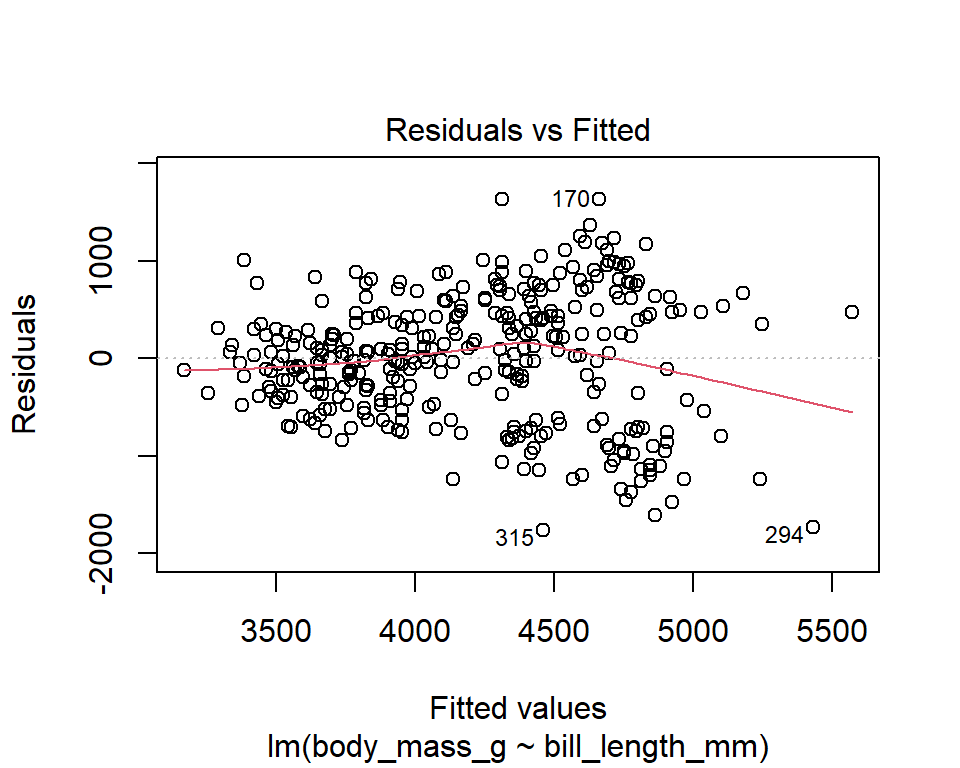
The diagnostic plots show residuals in four different ways. Let’s take a look at the first plot:
- Residuals vs Fitted
This plot shows the residuals (\(Y_i - \hat{Y}_i\)) on the y-axis and the fitted values (\(\hat{Y}_i\)) on the x-axis. If you find equally spread residuals around a horizontal line without distinct patterns, it is a good indication that the relationship between the variables can be considered linear. The red line is R’s attempt to capture any trends on the plot.
In our example above, there doesn’t seem to be signs of non-linearity in the residuals. However, it’s possible to see that the variability in the residuals tends to increase as the predicted values increase.
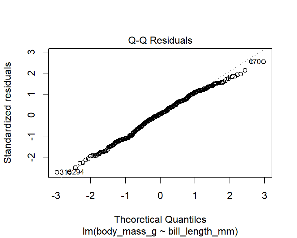
- Normal Q-Q plot
This plot shows the standardized residuals (y-axis) versus the theoretical quantiles (x-axis) for a normal distribution. If the points follow a straight line, then it is an indication that the residuals can be considered normally distributed. However, it’s usually the case that there’s some deviation from the line (especially towards the tails), especially in large samples. Only Q-Q plots that deviate in an obvious and consistent way from the line should be flagged. Alternatively, one may plot a histogram of the residuals to check for normality. For large samples, a violation of this condition is not as problematic because the CLT should “fix” this issue.
In our example, the points follow a straight line fairly well , which indicates that the residuals are consistent with a normal distribution. Let’s check this with a histogram:
data.frame(residuals = m1$residuals) |>
  ggplot(aes(x = residuals)) +
  geom_histogram(bins = 15, alpha = 0.3, color = "black")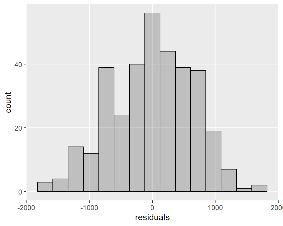
Note: When samples are large, deviations from normality are are not that concerning (this is a consequence of the Central Limit Theorem).
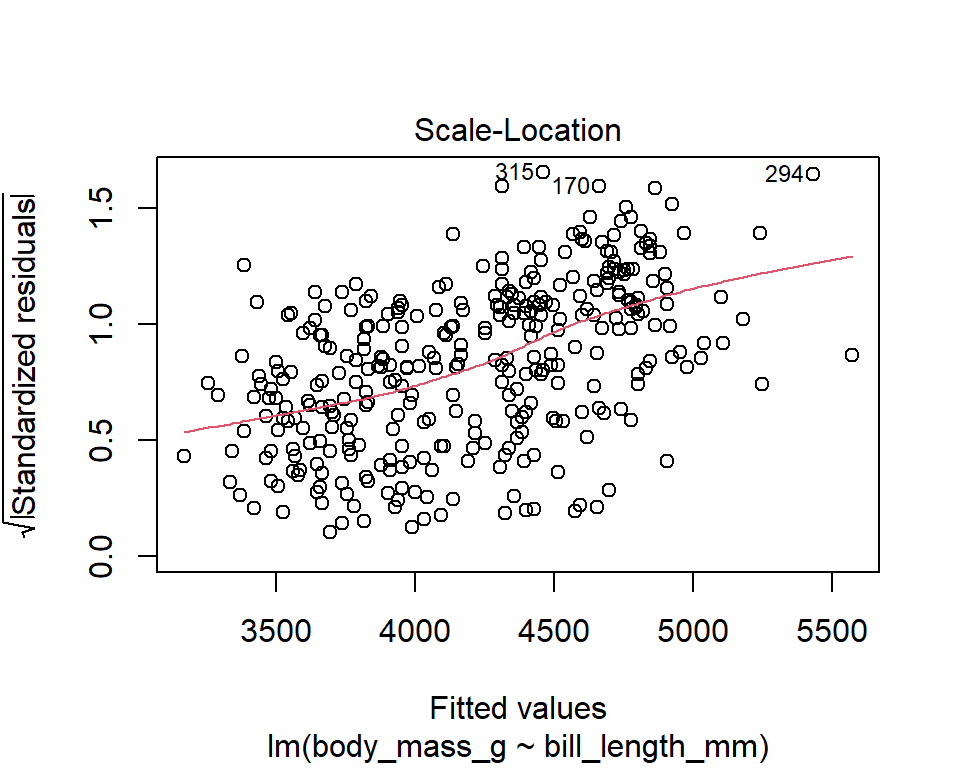
- Scale-Location plot
It’s also called Spread-Location plot. This plot shows whether residuals are spread equally along the ranges of predictors. This is how you can check the assumption of constant variance. It’s a good sign if you see a horizontal line with equally (randomly) spread points. In our example, residuals seem to have an increasing pattern in their variability (larger predicted values are associated with larger variability).
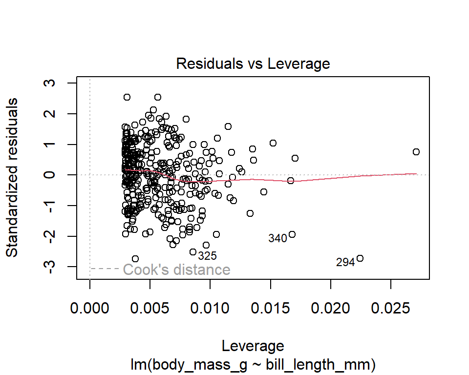
- Residuals vs Leverage
This plot helps us to find influential cases, if any. Not all outliers are influential in linear regression analysis. Even though data have extreme values, they might not be influential to determine a regression line. That means, the results wouldn’t be much different if we either include or exclude them from analysis. They follow the trend in the majority of cases and they don’t really matter; they are not influential. On the other hand, some cases could be very influential even if they look to be within a reasonable range of the values. They could be extreme cases against a regression line and can alter the results if we exclude them from analysis. Another way to put it is that they don’t get along with the trend in the majority of the cases.
The y-axis shows the standardized residuals. Points that are farther from zero have larger residuals, indicating that the model doesn’t fit these points well. The x-axis shows leverage, a measure of how far the predictors’ values are from the mean of all predictors. High-leverage points have the potential to exert more influence on the regression line. We watch out for outlying values at the upper right corner or at the lower right corner.
If dashed contour lines are present, they represent Cook’s distance, a measure of influence that considers both leverage and residual size. Points falling outside these contours have high Cook’s distance, indicating that they could disproportionately influence the regression model. Typically, points with Cook’s distance above 0.5 or 1 are considered influential. The regression results will likely be altered if we exclude those cases.
In our example, there are no influential outliers (no points beyond a Cook’s distance of 1.)
Independence condition
The four diagnostic plots can’t help us in a clear way on how to assess whether the errors are independent. In fact, there is no “definite” way for checking for independence. A first step it to check that the data collection was done in a way that avoided biases. For serial data (for example, data that were collected over time), we need to check whether future observations are dependent on previous ones. R’s acf (autocorrelation) function can help in this task. The acf function calculates Pearson correlations for a variable with its lagged values and it returns a plot of these autocorrelations along with a confidence band for them. If autocorrelations are high (beyond the confidence band), it is an indication that the values are dependent on previous values.
Conclusion for the penguins example:
For the model body_mass_g ~ bill_length_mm, we must take the results of the hypothesis tests for the slopes with caution, because “constant variability” condition seemed to be violated.
Sometimes, applying transformations to variables in the model can resolve some of the “bad” diagnostics.
11.3 Confidence interval for \(b\)
The sampling distributions from section 11.1.2 allow us to compute confidence intervals for \(b\) and \(a\) as follows: \[\begin{eqnarray} \mbox{CI for } b:& &\hat{b} \pm c\times SE(\hat{b})\\ \mbox{CI for } a:& &\hat{a} \pm c\times SE(\hat{a}) \end{eqnarray}\]
Such calculation is demonstrated in the following example.
Example 11.1 Suppose that we would like to find a confidence interval for the slope of the line that describes the relationship between body_mass_g and bill_length_mm in the penguins dataset. Let’s take another look at the summary table for the model:
## # A tibble: 2 × 5
##   term           estimate std.error statistic  p.value
##   <chr>             <dbl>     <dbl>     <dbl>    <dbl>
## 1 (Intercept)       362.     283.        1.28 2.02e- 1
## 2 bill_length_mm     87.4      6.40     13.7  3.81e-34
This gives
\[SE(\hat{b})=6.402\quad\mbox{and}\quad SE(\hat{a})=283.345.\]
For a 95% confidence interval, the critical value is \(c=qt(1-0.05/2, df),\) where \(df=n-2\). Even though the data has 344 rows, not all of them were necessarily used in computing the least squares model. This is because R excludes any rows that have a missing value for at least one of the variables. To check how many observations were actually included in the model, we can use the function glance from the broom package:
## [1] 340## [1] 342The last two columns in this summary give the degrees of freedom for the residuals (\(n-2 = 340\)) and the number of observations used in the model (\(n = 342\)). Now we can compute the critical value for a 95% confidence:
## [1] 1.966966Therefore, a 95% confidence interval for \(b\) is
\[\hat{b}\pm c\times SE(\hat{b}) = 87.415\pm 1.967\times 6.402 = [74.82, 100.01].\]
The confidence interval tells us that, with 95% confidence, the population slope \(b\) is between 74.82 and 100.01.
A confidence interval for the intercept can be calculated in a similar way; however, such interval is of much less interest than the one for the slope, as it is often the case that the intercept is not interpretable.
The calculations for confidence intervals described above are reasonable if assumptions A1 and A2 are met. We check for these assumptions through the diagnostic plots discussed in section 11.2.
11.4 Hypotheses testing for \(b\)
We would like to test the following hypotheses:
\(H_0: b = 0\)
\(H_a: b \neq 0\)
Recall that a non-zero slope is indicative of an existing relationship between the explanatory and the response variable.
Under the null hypothesis, the distribution of \(\hat{b}\) is
\[\hat{b} \sim N\left(0, \frac{\sigma}{\sqrt{\sum(X_i-\overline{X})^2}}\right).\]
Since we usually don’t have access to \(\sigma^2\), we use the MSE as an estimate for \(\sigma^2.\) The MSE is defined in section 11.5.1. When using this estimate, the t distribution should be used instead of the normal distribution. That is,
\[\frac{\hat{b}-0}{SE(\hat{b})} \sim t_{n-2},\] where \[SE(\hat{b}) \approx \sqrt{\frac{MSE}{\sum(X_i-\overline{X})^2}}.\]
This allows us to compute the test statistic for the hypothesis test: \[\begin{eqnarray} T = \frac{\hat{b}}{SE(\hat{b})}. \end{eqnarray}\] Then the p-value for the hypothesis test is the probability of observing this T statistic or more extreme, under the null hypothesis, that is, \[p-value = 2*pt(-|T|, df) = 2*(1-pt(|T|, df)),\] where \(df = n-2.\) Such calculation is demonstraded in the following example.
Example 11.2 Suppose that we would like to find the significance of the slope of the line that describes the relationship between body_mass_g and bill_length_mm in the penguins dataset.
The test statistic is 87.415 \[T = \frac{\hat{b}}{SE(\hat{b})} = \frac{87.415}{6.402} = 13.65,\] which gives the p-value: \[p-value = 2*(1-pt(13.65, df = 340)) \approx 0.\] Since the p-value is less than the significance level \(\alpha=0.05,\) we can reject the null hypothesis and conclude that there is strong evidence that the true slope of the line is not zero. In this case, the data sugest that there is a positive association between body mass and bill length.
A hypothesis test for the intercept can be carried out in a similar way; however, such test is of much less interest than the one for the slope, as it is often the case that the intercept is not interpretable.
The calculations for hypothesis testing described above are reasonable if assumptions A1 and A2 are met. We check for these assumptions through the diagnostic plots discussed in section 11.2.
11.5 Analysis of variance (ANOVA)
Analysis of variance, or in short, ANOVA, is a way of analyzing relationships by partitioning the variability of a response variable into appropriate “sums of squares” for analysis.
11.5.1 ANOVA for one predictor
Let’s consider one numerical response variable and one explanatory variable (numerical or categorical with two levels). We will later describe how this changes when considering more explanatory variables. For a sample with \(n\) observations, write each observation for the two variables as \((X_1, Y_1), (X_2, Y_2), \dots, (X_n, Y_n)\). If appropriate, we can fit a least squares model to these two variables.
First, we recall important quantities in regression analysis, the residuals.
Definition 11.1 Consider a regression model that estimates \(Y_i\) with \(\hat{Y}_i\). The residuals of the regression model, denoted by \(\hat{e}\), is the error of the estimate \(\hat{Y}_i\).That is, \(\hat{e} = Y_i - \hat{Y}_i\).
Recall that we denoted by \(SS(a,b)\) the sum of the squares of the vertical distances \(Y_i - (a + bX_i)\), that is, \(SS(a,b) = \sum (Y_i - (a + bX_i))^2\). For a least squares model \(\hat{Y}_i = \hat{a} + \hat{b} X_i\), the quantity \(SS(\hat{a},\hat{b})\) is the sum of the squares of the residuals, which is the smallest possible value of \(SS(a,b)\) (see definition 3.1). We call this quantity SSE, which stands for “Sum of Squares Error”. Another quantity of interest is \(SS(\overline{Y},0) = \sum(Y_i - \overline{Y})^2\), the total sum of squares of \(Y_i\) about \(\overline{Y}\). We name this quantity SST, which stands for “Sum of Squares Total” and represents the total variability of the response variable about its mean (how does this resemble definition 2.5?31.) These definitions are summarized below.
Definition 11.2 The “Sum of Squares Error” is defined as \[SSE = SS(\hat{a}, \hat{b}) = \sum(Y_i - (\hat{a} +\hat{b}X_i))^2 = \sum(Y_i - \hat{Y}_i)^2,\] and the “Sum of Squares Total” is defined as \[SST = SS(\overline{Y}, 0) = \sum(Y_i - \overline{Y})^2.\]
Notice that the following inequality holds: \(SSE \leq SST\). This is because SSE is the smallest possible value for \(SS(a,b)\), so it must not be greater than \(SS(\overline{Y}, 0) = SST\). This means that we can write
\[SST = SSE + \mbox{something non-negative}.\]
To find what that “something non-negative” is, we begin with SST and try to re-write it in a way that includes SSE. We accomplish this by subtracting and adding \(\hat{Y}_i\) within the expression for SST and expanding it:
\[\begin{eqnarray} SST &=& \sum(Y_i - \overline{Y})^2 = \sum(Y_i - \hat{Y}_i + \hat{Y}_i - \overline{Y})^2 = \sum((Y_i - \hat{Y}_i) + (\hat{Y}_i - \overline{Y}))^2\\ &=& \sum\left[(Y_i - \hat{Y}_i)^2 + 2(Y_i - \hat{Y}_i)(\hat{Y}_i - \overline{Y}) + (\hat{Y}_i - \overline{Y})^2\right]\\ &=& \sum(Y_i - \hat{Y}_i)^2 + 2\sum(Y_i - \hat{Y}_i)(\hat{Y}_i - \overline{Y}) + \sum(\hat{Y}_i - \overline{Y})^2. \end{eqnarray}\]
It turns out that \(\sum(Y_i - \hat{Y}_i)(\hat{Y}_i - \overline{Y}) = 0\)32, which gives
\[\sum(Y_i - \overline{Y})^2 = \sum(Y_i - \hat{Y}_i)^2 + \sum(\hat{Y}_i - \overline{Y})^2.\] This equation shows a partition of SST into two sums of squares. The quantity \(\sum(\hat{Y}_i - \overline{Y})^2\) is called the “Sum of Squares Regression”, or SSR. In short,
\[SST = SSE + SSR.\]
Each of these quantities tell us something about the LS model. For instance, \(SSR = 0\) if (and only if) \(\hat{Y}_i = \overline{Y}\). That is, \(\hat{b} = 0\) and \(\hat{a} = \overline{Y}\). This is a horizontal LS line, which is usually an indication that the variables \(X\) and \(Y\) are not associated and that the variable \(X\) does not help predict \(Y\) any more than \(\overline{Y}\) predicts \(Y\). So we can say that the lower the value of SSR, the worse the LS fit. On the other hand, the higher the SSR, the better the fit. In summary,
\[\begin{eqnarray} & & \mbox{lower SSR (higher SSE)} \rightarrow \mbox{ worse fit}\\ & & \mbox{higher SSR (lower SSE)} \rightarrow \mbox{ better fit}. \end{eqnarray}\]
Looking at the expressions for SST and SSE, we can see that adding more points in the dataset will increase SST and SSE (because we are adding more squared terms).
For any sum of squares, the mean square (MS) is defined as \(\frac{SS}{df}\), where \(df\) are the degrees of freedom of the sum of squares. We won’t provide a through treatment of degrees of freedom here, but roughly speaking, the degrees of freedom of an expression are number of variables in the expression minus the number of equations they satisfy. When there’s only one predictor, the degrees of freedom for SST, SSR, and SSE are \(n-1\), 1, and \(n-2\) respectively. Therefore, the “Mean Square Total”, “Mean Square Regression”, and “Mean Square Error” are given by:
\[MST = SST/(n-1), \quad MSR = SSR/1, \quad \mbox{and} \quad MSE = SSE/(n-2).\]
Notice that \(df(SST) = df(SSR) + df(SSE)\). It may not be clear at this point why the mean squares are particularly useful, but we will see that they play an important role in statistical inference. The sums of squares and mean squares are all summarized in an analysis of variance (ANOVA) table. In R, the ANOVA table can be obtained by applying the anova function to a least squares model. For example, using the county dataset from the openintro package (see section 1.2 for a description of the variables in the data), let’s fit a least squares model that predicts population change from median household income and print the ANOVA table for the model.
ANOVA table for the least squares model pop_change ~ median_hh_income:
##
## Call:
## lm(formula = pop_change ~ median_hh_income, data = county)
##
## Coefficients:
##      (Intercept)  median_hh_income
## -5.7712741 0.0001267## Analysis of Variance Table
##
## Response: pop_change
## Df Sum Sq Mean Sq F value Pr(>F)
## median_hh_income 1 8706 8706.5 625.66 < 2.2e-16 ***
## Residuals 3135 43625 13.9
## ---
## Signif. codes: 0 '***' 0.001 '**' 0.01 '*' 0.05 '.' 0.1 ' ' 1The table excludes the sum of squares and mean squares for the total. This is because that information can be obtained from SSR and SSE.
The first column of the table has the degrees of freedom for SSR and SSE;
The second column of the table has SSR and SSE;
The third column of the table has MSR and MSE;
The “F Value” is a statistic used for carrying out a hypothesis test for the following hypotheses:
\(H_0\) (null hypothesis): A model with median household income as a predictor is not an improvement over a model with no predictors.33
\(H_a\) (alternative hypothesis): A model with median household income as a predictor is an improvement over the model with no predictors.
- The quantity “Pr(>F)” is the p-value for the hypotheses stated above. A p-value that is “small enough”34 is evidence against the null hypothesis, in favor of the alternative.
11.5.2 Coeficient of determination
The coefficient of determination is a quantity that can be used to evaluate the strength of a linear fit. It is defined as follows.
Definition 11.3 The coefficient of determination is defined as \[R^2 = \frac{SSR}{SST} = 1 - \frac{SSE}{SST}.\] It is the proportion of SST apportioned to the regression. It is seen as the proportion of the variability in \(Y\) that is explained by the model.
The coefficient of determination is always a number greater than or equal to 0 and less than or equal to 1.
When \(R^2=1\), there’s a perfect fit (all data points are on the LS line). In this case, \(SSR=SST\) and \(SSE=0\).
When \(R^2 = 0\), there’s complete lack of fit. In this case, \(SST=SSE\) and \(SSR=0\).
Larger values of \(R^2\) correspond to better fits.
\(R^2\) is the square of Pearson’s correlation coefficient.
Example 11.3 From the ANOVA table for The model pop_change ~ median_hh_income, we have that \(SSR = 34234\), \(SSE = 111005\), and \(SST = SSR + SSE = 34234 + 111005 = 145239\). The coefficient of determination for the model is \[R^2 = 1-\frac{111005}{145239} = 0.2357.\]
So we can say that the model explains 23.57% of the variability in population percent change. This is considered to be a weak association.
11.5.3 ANOVA for more than one predictor
In section 11.5.1, we looked at how to partition the total variability of the response variable, SST, into two sums of squares, SSR + SSE. This partition also holds for multiple least squares regression; however, the degrees of freedom for each sum of squares change to account for the addition of variables. For a model with \(k\) predictors, built with a sample of size \(n\), the degrees of freedom for SST, SSR, and SSR are:
\[df(SST) = n-1, \quad df(SSR) = k, \quad df(SSE) = n-k-1.\]
Therefore,
\[MST = \frac{SST}{n-1}, \quad MSR = \frac{SSR}{k}, \quad MSE = \frac{SSE}{n-k-1}.\]
Let’s look at the ANOVA table for the model interest_rate ~ annual_income + debt_to_income + bankruptcy + verified_income from the loans_full_schema dataset in the openintro package:
library(openintro)
library(tidyverse)
loans <- loans_full_schema
loans <- mutate(loans, bankruptcy = if_else(public_record_bankrupt == 0, "no", "yes"))
m <- lm(interest_rate ~ annual_income + debt_to_income + bankruptcy + verified_income, data = loans)
anova(m)
## Analysis of Variance Table
##
## Response: interest_rate
## Df Sum Sq Mean Sq F value Pr(>F)
## annual_income 1 2427 2427.5 105.868 < 2.2e-16 ***
## debt_to_income 1 3950 3950.1 172.270 < 2.2e-16 ***
## bankruptcy 1 487 487.4 21.255 4.071e-06 ***
## verified_income 2 13694 6846.8 298.601 < 2.2e-16 ***
## Residuals 9970 228607 22.9
## ---
## Signif. codes: 0 '***' 0.001 '**' 0.01 '*' 0.05 '.' 0.1 ' ' 1Here we see sums of squares for each variable; adding all of them gives SSR. In this case, \(SSR = 2427 + 3950 + 487 + 13694 = 20558\) and \(SSE = 228607\). This form of reporting SSR is called sequential sum of squares. This list shows us how much SSR increases as we add each of the predictor variables in turn. Since SST is the same no matter how many variables we have in the model, the increase in SSR helps us judge how important a variable may be.
If we only included the variable annual_income in the model, then SSR would be 2427. If we then add debt_to_income, making it a model with two predictors, SSR increases by 3950. Similarly, if we then add bankruptcy, SSR increases by 487. Finally, if we then add verified_income, SSR increases by 13694. The increases in SSR depend on the order in which we add the variables to the model. If annual_income was the second variable entered instead of the first, the sequential sum of squares would be different. In summary, the sum of squares listed for a variable gives the increase in SSR once all the previous variables are in the model. However, SSR is always the same for a model with these 4 predictors, regardless of the order in which they are entered.
As in the case for the ANOVA table with one predictor, there are also F values and p-values. To give an example, the hypotheses that are being tested for the variable bankruptcy are the following:
\(H_0\) (null hypothesis): Adding bankruptcy to a model that has annual income and debt_to_income does not improve the existing model.
\(H_a\) (alternative hypothesis): Adding bankruptcy to a model that has annual income and debt_to_income improves the existing model.
To end this example, the sum of squares and mean squares in the ANOVA table are given by:
\(SSR = 20558, \, SSE = 228607, \, SST = 20558 + 228607 = 249165.\)
\(MST = \frac{SST}{n-1} = \frac{249165}{9975} = 24.98, \, MSR = \frac{SSR}{k} = \frac{20558}{5} = 4111.6, \, MSE = \frac{SSE}{n-k-1} = \frac{228607}{9970} = 22.93.\)
The denominators are the degrees of freedom in the first column (for SSR, we sum the degrees of freedom for the sequential sum of squares). Notice that even though we are adding 4 variables to the model, the degrees of freedom for SSR is 5. This is because the variable verified_income, when added to the model, generates two indicator variables, making the model have 5, instead of 4 variables. It should also be noted that SST and MST do not appear in the ANOVA table.
11.5.4 ANOVA for categorical predictors
One of the most common uses of an ANOVA is to serve as a “gateway” test for whether categorical predictors are significantly related to numerical responses. For example, we may want to know whether the body mass of penguins in the Palmer Archipelago, Antarctica, differ by species. We can fit a linear model to address this scenario:
## # A tibble: 3 × 5
##   term             estimate std.error statistic   p.value
##   <chr>               <dbl>     <dbl>     <dbl>     <dbl>
## 1 (Intercept)        3701.       37.6    98.4   2.49e-251
## 2 speciesChinstrap     32.4      67.5     0.480 6.31e-  1
## 3 speciesGentoo      1375.       56.1    24.5   5.42e- 77
The model gives comparisons with a reference level, in this case, the Adelie species. We can conclude that penguins from the Gentoo species tend to have higher body mass than the Adelie species, by an average of 1375.35 g. This difference is statistically significant (p-value < 0.05). The body mass of penguins in the Chinstrap species is not statistically different than the Adelie species (p-value > 0.05).
Comparing a group’s mean to a reference level may fall short of fully addressing differences among 3 or more groups if there is no particular reason to only look at comparisons with one reference group. For instance, we may be just as interested in knowing whether the Gentoo and Chinstrap species differ in average body mass. A more common sequence of tests for this scenario is to first perform an ANOVA as a “gateway” test, that is, a test for weather body mass varies by species, and if so, do follow up tests to assess which species have (statistically) different body mass. These steps can be carried out as follows:
- Look at an ANOVA table of the model
body_mass_g ~ species:
## Analysis of Variance Table
##
## Response: body_mass_g
##            Df    Sum Sq  Mean Sq F value    Pr(>F)
## species     2 146864214 73432107  343.63 < 2.2e-16 ***
## Residuals 339  72443483   213698
## ---
## Signif. codes:  0 '***' 0.001 '**' 0.01 '*' 0.05 '.' 0.1 ' ' 1
The ANOVA tells us that species is a statistically significant predictor of body mass. This means that the penguins’ average body mass is likely not the same across species (otherwise the variable species would not be a significant predictor). In other words, the null and alternative hypotheses for an ANOVA’s F-test are equivalent to:
\(H_0:\) The penguins’ mean body mass does not vary by species (all species have the same mean).
\(H_a:\) The penguins’ mean body mass varies by species (at least one pair of means differ).
When we reject this null hypothesis, a natural follow-up question is “which means differ?” One way to address this question is to to pairwise comparisons for the difference between two means using the hypothesis test introduced in section 10.4. In the current example, we would need three pairwise tests.
In R, this can be accomplished with the function pairwise_t_test() from the package rstatix, as follows:
## # A tibble: 3 × 9
##   .y.         group1  group2    n1    n2        p p.signif    p.adj p.adj.signif
## * <chr>       <chr>   <chr>  <int> <int>    <dbl> <chr>       <dbl> <chr>
## 1 body_mass_g Adelie  Chins…   152    68 6.31e- 1 ns       6.31e- 1 ns
## 2 body_mass_g Adelie  Gentoo   152   124 5.42e-77 ****     1.63e-76 ****
## 3 body_mass_g Chinst… Gentoo    68   124 3.21e-56 ****     6.42e-56 ****
The p-values in the column p.adj are “adjusted” for multiple testing, whereas the ones in column p are the original ones. The adjusted p-values make it easier to control for false discoveries. More specifically, for a significance level \(\alpha\), the adjustment is such that the probability of incorrectly rejecting the null hypothesis in at least one of the three tests above is not more than \(\alpha\). Without the adjustment, this probability would be larger than \(\alpha\) (and would increase the possibility of making a false discovery). The most conservative35 adjustment is to multiply the original p-values in the pairwise comparisons by the total number of comparisons being made (in this example, 3). This is Bonferroni’s correction.
A less conservative adjustment is Holm’s correction, which is the default adjustment in the function pairwise_t_test(). Holm’s correction works by ordering all p-values from smallest (\(p_{(1)}\)) to largest (\(p_{(m)}\)) for \(m\) tests, then multiplying each \(p_{(i)}\) by \(m - i + 1\).
This method is statistically more powerful than Bonferroni correction while still controlling for multiple comparisons.
Going back to the pairwise comparisons, they indicate that Gentoo’s mean body mass differs from that of Adelie’s and Chinstrap’s. Specifically, Gentoo penguins tend to be heavier.
11.5.5 Adjusted R-squared
The coefficient of determination, \(R^2\) can also be calculated in a multiple linear regression model. For the model in the previous subsection,
\[R^2 = 1 - \frac{SSE}{SST} = 1 - \frac{228607}{249165} = 0.0825,\]
which can be interpreted as 8.25% of the variability in interest rate is explained by the model. This is a low \(R^2\), indicating that adding more variables could possibly help account for unexplained variablity. However, using \(R^2\) as a tool to decide whether to add more variables can be problematic because \(R^2\) always increases when we add more variables, even if by just a tiny amount. A better measure for model selection is a variation of \(R^2\), called “adjusted \(R^2\)”. This adjusted measure replaces SSE and SST with MSE and MST in the formula for \(R^2\).
Definition 11.4 The adjusted coefficient of determination, or adjusted \(R^2\), is defined as \[R^2_{adj} = 1-\frac{MSE}{MST} = 1 - \frac{SSE/(n-k-1)}{SST/(n-1)}.\]
Notice that \(R^2_{adj} \leq R^2\) (is it clear why?). Further, \(R^2_{adj}\) can decrease if we add too many variables that don’t significantly improve the model. Therefore, a simple way to use \(R^2_{adj}\), is to not add a variable to a model if that variable causes a decrease in \(R^2_{adj}\).
For the model with 4 variables developed above,
\[R^2_{adj} = 1 - \frac{MSE}{MST} = 1 - \frac{22.93}{24.98} = 0.0821,\]
Both \(R^2\) and \(R^2_{adj}\) can be obtained through the glance function from the broom package:
| r.squared | adj.r.squared | sigma | statistic | p.value | df | logLik | AIC | BIC | deviance | df.residual | nobs |
|---|---|---|---|---|---|---|---|---|---|---|---|
| 0.669672 | 0.6677231 | 462.2744 | 343.6263 | 0 | 2 | -2582.337 | 5172.673 | 5188.012 | 72443483 | 339 | 342 |
We will cover strategies to perform model selection in the next section.
11.6 Model selection
The best model is not always the most complicated. Sometimes including variables that are not evidently important can actually reduce the accuracy of predictions. In this section, we discuss model selection strategies, which will help us eliminate variables from the model that are found to be less important. It’s common (at least in the statistical world) to refer to models that have undergone such variable pruning as parsimonious.
In practice, the model that includes all available explanatory variables of interest is often referred to as the full model. The full model may not be the best model, and if it isn’t, we want to identify a smaller model that is preferable.
The adjusted \(R^2\) measures the strength of a model fit, and it is a useful tool for evaluating which predictors are adding value to the model, where adding value means they are (likely) improving the accuracy in predicting future outcomes.
Two common strategies for adding or removing variables in a multiple regression model are called backward elimination and forward selection. These techniques are often referred to as step- wise model selection strategies, because they add or delete one variable at a time as they “step” through the candidate predictors.
11.6.1 Backward elimination
Backward elimination starts with the model that includes all potential predictor variables. Then variables are eliminated one-at-a-time from the model until we cannot improve the adjusted \(R^2\). The strategy within each elimination step is to eliminate the variable that leads to the largest improvement in adjusted \(R^2\).
To fit an LS model using all predictors available in a dataset, one can use the syntax lm(y ~ .), which means fit a model that has y as the response and all other variables in the dataset as predictors. Let’s return to the loans dataset and consider the following 15 predictors (instead of only 4 predictors):
“homeownership”, “annual_income”, “bankruptcy”, “verified_income”, “debt_to_income”, “delinq_2y”, “months_since_last_delinq”, “earliest_credit_line”, “inquiries_last_12m”, “total_credit_lines”, “open_credit_lines”, “total_credit_limit”, “total_credit_utilized”, “term”, “current_installment_accounts”.
To make coding easier, we can define a new dataset with only these variables plus interest_rate. Let’s call this dataset loans2:
loans2 <- loans[, c("homeownership", "annual_income", "bankruptcy", "verified_income", "debt_to_income", "delinq_2y", "months_since_last_delinq", "earliest_credit_line", "inquiries_last_12m", "total_credit_lines", "open_credit_lines", "total_credit_limit", "total_credit_utilized", "term", "current_installment_accounts", "interest_rate")]The code above selects the columns of the loans dataset, by name, that will be part of the new dataset.
Now we can obtain the full model for interest_rate by running:
## # A tibble: 18 × 5
##    term                               estimate    std.error statistic   p.value
##    <chr>                                 <dbl>        <dbl>     <dbl>     <dbl>
##  1 (Intercept)                    -92.7        18.6            -5.00  6.07e-  7
##  2 homeownershipOWN                 0.384       0.208           1.84  6.58e-  2
##  3 homeownershipRENT                0.400       0.166           2.41  1.58e-  2
##  4 annual_income                   -0.00000181  0.00000111     -1.63  1.04e-  1
##  5 bankruptcyyes                    0.555       0.234           2.37  1.77e-  2
##  6 verified_incomeSource Verified   0.868       0.149           5.82  6.37e-  9
##  7 verified_incomeVerified          2.15        0.179          12.0   8.90e- 33
##  8 debt_to_income                   0.0528      0.00526        10.0   2.01e- 23
##  9 delinq_2y                        0.341       0.0821          4.16  3.24e-  5
## 10 months_since_last_delinq        -0.0189      0.00365        -5.19  2.25e-  7
## 11 earliest_credit_line             0.0492      0.00926         5.31  1.15e-  7
## 12 inquiries_last_12m               0.247       0.0271          9.13  1.07e- 19
## 13 total_credit_lines              -0.0407      0.00878        -4.63  3.73e-  6
## 14 open_credit_lines                0.00362     0.0178          0.203 8.39e-  1
## 15 total_credit_limit              -0.00000437  0.000000473    -9.25  3.51e- 20
## 16 total_credit_utilized            0.00000695  0.00000168      4.13  3.72e-  5
## 17 term                             0.160       0.00597        26.9   2.87e-147
## 18 current_installment_accounts     0.0342      0.0273          1.25  2.11e-  1
The values of \(R^2\) and \(R^2_{adj}\) are:
## [1] 0.2568993## [1] 0.2539703Their values are quite similar, with \(R^2\) being just slightly higher than \(R^2_adj\) (recall that \(R^2_adj\) is never larger than \(R^2\)). Now we can experiment with trying to reduce this model to one with 14 predictors instead of 15. To decide which predictor should be eliminated, we can exclude a predictor and check how that exclusion changes the value of \(R^2_{adj}\). We record the changes in \(R^2_{adj}\) caused by excluding each variable. The variable that causes the highest increase in \(R^2_{adj}\) when eliminated, should be the first to be excluded. For example, if we eliminate open_credit_lines from the model, then \(R^2_{adj}\) becomes:
## [1] 0.2541361Notice that this value of \(R^2_{adj}\) is larger than the one for the full model. This means that eliminating open_credit_lines is not much of a loss to the model. So we check the changes in \(R^2_{adj}\) for all the other variables and eliminate the one that causes \(R^2_{adj}\) to increase the most. Then once we have a model with 13 variables, we proceed to check whether we can eliminate one more variable by going through the same procedure described above. I won’t make you “watch” this entire process, but the process ends when the elimination of any variable would lead to a decrease in \(R^2_{adj}\).
This process is called backward elimination because we begin with a full model and then proceed to eliminate variables that don’t contribute much to the model.
This process can be used with any other measure of fit; it is not exclusive to \(R^2_{adj}\). For instance, we could have used the p-values instead and started by eliminating the variable with the largest p-value, then re-fitting the model, then eliminating the variable with the largest p-value in the re-fitted model, and so on, until all p-values are “small enough”.
One of the most popular measures used in model selection is the AIC, which stands for Akaike Information Criterion. Its formal definition is beyond the scope of this course, but it can be used in a similar manner as \(R^2_{adj}\), with the difference that a lower AIC is better (in contrast to a higher \(R^2_{adj}\) being better). The value of AIC is highly dependent on the data, and it is not a number bounded by 1, like \(R^2_{adj}\). The default implementation in R for model selection is the step function, which uses the AIC as a criterion for eliminating or adding variables. That is, at each step, we eliminate the variable that decreases the AIC the most.
When running the step function, we need to ensure that the dataset comprised of all predictors and the response variable have no missing values (otherwise the function returns an error). We can accomplish this by applying na.omit to the dataset, as shown below:
full2 <- lm(interest_rate ~., data = na.omit(loans2))
reduced <- step(full2, direction = "backward")
## Start: AIC=12545.55
## interest_rate ~ homeownership + annual_income + bankruptcy +
## verified_income + debt_to_income + delinq_2y + months_since_last_delinq +
## earliest_credit_line + inquiries_last_12m + total_credit_lines +
## open_credit_lines + total_credit_limit + total_credit_utilized +
## term + current_installment_accounts
##
## Df Sum of Sq RSS AIC
## - open_credit_lines 1 0.7 77803 12544
## - current_installment_accounts 1 28.2 77831 12545
## <none> 77802 12546
## - annual_income 1 47.8 77850 12546
## - homeownership 2 125.2 77928 12548
## - bankruptcy 1 101.6 77904 12549
## - total_credit_utilized 1 307.5 78110 12561
## - delinq_2y 1 312.2 78115 12561
## - total_credit_lines 1 387.0 78189 12565
## - months_since_last_delinq 1 485.2 78288 12570
## - earliest_credit_line 1 508.7 78311 12572
## - inquiries_last_12m 1 1502.4 79305 12626
## - total_credit_limit 1 1542.8 79345 12629
## - debt_to_income 1 1815.1 79618 12643
## - verified_income 2 2608.5 80411 12684
## - term 1 13032.8 90835 13214
##
## Step: AIC=12543.59
## interest_rate ~ homeownership + annual_income + bankruptcy +
## verified_income + debt_to_income + delinq_2y + months_since_last_delinq +
## earliest_credit_line + inquiries_last_12m + total_credit_lines +
## total_credit_limit + total_credit_utilized + term + current_installment_accounts
##
## Df Sum of Sq RSS AIC
## - current_installment_accounts 1 35.3 77839 12544
## <none> 77803 12544
## - annual_income 1 47.5 77851 12544
## - homeownership 2 125.9 77929 12547
## - bankruptcy 1 102.1 77905 12547
## - total_credit_utilized 1 307.3 78110 12559
## - delinq_2y 1 311.5 78115 12559
## - months_since_last_delinq 1 486.2 78289 12569
## - earliest_credit_line 1 508.5 78312 12570
## - total_credit_lines 1 608.8 78412 12575
## - inquiries_last_12m 1 1515.6 79319 12625
## - total_credit_limit 1 1545.0 79348 12627
## - debt_to_income 1 1834.6 79638 12642
## - verified_income 2 2610.4 80414 12682
## - term 1 13032.6 90836 13212
##
## Step: AIC=12543.56
## interest_rate ~ homeownership + annual_income + bankruptcy +
## verified_income + debt_to_income + delinq_2y + months_since_last_delinq +
## earliest_credit_line + inquiries_last_12m + total_credit_lines +
## total_credit_limit + total_credit_utilized + term
##
## Df Sum of Sq RSS AIC
## <none> 77839 12544
## - annual_income 1 53.3 77892 12544
## - homeownership 2 131.5 77970 12547
## - bankruptcy 1 102.4 77941 12547
## - delinq_2y 1 310.1 78149 12559
## - total_credit_utilized 1 443.7 78282 12566
## - months_since_last_delinq 1 486.4 78325 12568
## - earliest_credit_line 1 559.5 78398 12573
## - total_credit_lines 1 573.7 78412 12573
## - inquiries_last_12m 1 1506.0 79345 12625
## - total_credit_limit 1 1571.1 79410 12628
## - debt_to_income 1 1871.0 79710 12644
## - verified_income 2 2599.6 80438 12682
## - term 1 13099.6 90938 13215Notice that the step function took the following steps:
First it eliminated
open_credit_linesbecause this reduced the AIC the most (from 12545.55 to 12544).Then it re-fit the model without
open_credit_linesand looked for which variable decreased the AIC the most. That variable wascurrent_installment_accounts, which was then eliminated.Then it re-fit the previous model without
current_installment_accountsand looked for which variable decreased the AIC the most. No such variable was found, so the procedure stopped.
The final reduced model was:
## # A tibble: 16 × 5
##    term                               estimate    std.error statistic   p.value
##    <chr>                                 <dbl>        <dbl>     <dbl>     <dbl>
##  1 (Intercept)                    -96.4        18.4             -5.25 1.58e-  7
##  2 homeownershipOWN                 0.385       0.208            1.85 6.46e-  2
##  3 homeownershipRENT                0.413       0.166            2.49 1.26e-  2
##  4 annual_income                   -0.00000191  0.00000111      -1.72 8.58e-  2
##  5 bankruptcyyes                    0.557       0.234            2.38 1.73e-  2
##  6 verified_incomeSource Verified   0.869       0.149            5.83 6.07e-  9
##  7 verified_incomeVerified          2.15        0.179           12.0  1.14e- 32
##  8 debt_to_income                   0.0533      0.00523         10.2  4.35e- 24
##  9 delinq_2y                        0.340       0.0820           4.15 3.45e-  5
## 10 months_since_last_delinq        -0.0189      0.00365         -5.19 2.17e-  7
## 11 earliest_credit_line             0.0510      0.00917          5.57 2.72e-  8
## 12 inquiries_last_12m               0.247       0.0270           9.14 9.67e- 20
## 13 total_credit_lines              -0.0371      0.00657         -5.64 1.82e-  8
## 14 total_credit_limit              -0.00000440  0.000000471     -9.33 1.61e- 20
## 15 total_credit_utilized            0.00000776  0.00000156       4.96 7.35e-  7
## 16 term                             0.161       0.00597         26.9  5.78e-148
Notice that not all variables in the final model are statistically significant. If this is an important aspect of a desirable final model, then you could proceed to further eliminate variables.
11.6.2 Forward selection
The forward selection strategy is the reverse of the backward elimination technique. Instead of eliminating variables one-at-a-time, we add variables one-at-a-time until we cannot find any variables that improve the model (as measured by \(R^2_{adj}\), or AIC, or p-value, etc).
Backward elimination and forward selection sometimes arrive at different final models. For the previous example, a forward selection strategy gives:
min.model <- lm(interest_rate ~ 1, data = na.omit(loans2))
full_formula <- formula(full2)
reduced_f <- step(min.model, direction = "forward", scope = full_formula)
## Start: AIC=13797.53
## interest_rate ~ 1
##
## Df Sum of Sq RSS AIC
## + term 1 13089.7 91610 13221
## + verified_income 2 5030.8 99669 13588
## + debt_to_income 1 2476.2 102224 13696
## + total_credit_limit 1 1785.0 102915 13725
## + inquiries_last_12m 1 1400.8 103299 13741
## + earliest_credit_line 1 1351.9 103348 13743
## + annual_income 1 1332.6 103367 13744
## + months_since_last_delinq 1 702.7 103997 13770
## + delinq_2y 1 585.8 104114 13775
## + homeownership 2 519.2 104181 13780
## + current_installment_accounts 1 335.2 104365 13786
## + total_credit_lines 1 225.3 104474 13790
## + bankruptcy 1 163.6 104536 13793
## <none> 104700 13798
## + total_credit_utilized 1 29.1 104671 13798
## + open_credit_lines 1 10.3 104689 13799
##
## Step: AIC=13221.1
## interest_rate ~ term
##
## Df Sum of Sq RSS AIC
## + verified_income 2 3209.4 88401 13071
## + total_credit_limit 1 2950.5 88660 13081
## + debt_to_income 1 2374.4 89236 13109
## + annual_income 1 1657.7 89952 13144
## + earliest_credit_line 1 1567.2 90043 13148
## + homeownership 2 1267.8 90342 13165
## + inquiries_last_12m 1 1198.7 90411 13166
## + months_since_last_delinq 1 947.7 90662 13178
## + delinq_2y 1 833.1 90777 13184
## + total_credit_lines 1 560.9 91049 13196
## + bankruptcy 1 209.7 91400 13213
## + current_installment_accounts 1 116.2 91494 13218
## + open_credit_lines 1 97.1 91513 13218
## <none> 91610 13221
## + total_credit_utilized 1 13.6 91596 13222
##
## Step: AIC=13070.65
## interest_rate ~ term + verified_income
##
## Df Sum of Sq RSS AIC
## + total_credit_limit 1 3555.2 84845 12895
## + debt_to_income 1 1857.7 86543 12981
## + annual_income 1 1728.7 86672 12987
## + homeownership 2 1579.6 86821 12997
## + earliest_credit_line 1 1521.3 86879 12998
## + inquiries_last_12m 1 958.3 87442 13025
## + months_since_last_delinq 1 844.2 87556 13031
## + delinq_2y 1 755.4 87645 13036
## + total_credit_lines 1 554.2 87846 13045
## + bankruptcy 1 190.3 88210 13063
## + open_credit_lines 1 118.1 88283 13067
## + current_installment_accounts 1 116.6 88284 13067
## + total_credit_utilized 1 42.8 88358 13071
## <none> 88401 13071
##
## Step: AIC=12894.87
## interest_rate ~ term + verified_income + total_credit_limit
##
## Df Sum of Sq RSS AIC
## + debt_to_income 1 2085.47 82760 12789
## + inquiries_last_12m 1 1413.29 83432 12824
## + months_since_last_delinq 1 1084.38 83761 12841
## + delinq_2y 1 938.62 83907 12849
## + earliest_credit_line 1 798.09 84047 12856
## + total_credit_utilized 1 685.40 84160 12862
## + current_installment_accounts 1 393.87 84452 12877
## + annual_income 1 154.60 84691 12889
## + homeownership 2 175.57 84670 12890
## + bankruptcy 1 84.60 84761 12892
## <none> 84845 12895
## + total_credit_lines 1 27.61 84818 12896
## + open_credit_lines 1 25.52 84820 12896
##
## Step: AIC=12789.09
## interest_rate ~ term + verified_income + total_credit_limit +
## debt_to_income
##
## Df Sum of Sq RSS AIC
## + inquiries_last_12m 1 1361.15 81399 12719
## + months_since_last_delinq 1 1206.32 81554 12728
## + delinq_2y 1 1034.24 81726 12737
## + earliest_credit_line 1 1011.24 81749 12738
## + total_credit_utilized 1 254.95 82505 12778
## + total_credit_lines 1 217.38 82543 12780
## + homeownership 2 230.48 82530 12781
## + current_installment_accounts 1 125.47 82635 12784
## + bankruptcy 1 89.19 82671 12786
## <none> 82760 12789
## + open_credit_lines 1 24.84 82735 12790
## + annual_income 1 2.16 82758 12791
##
## Step: AIC=12719.26
## interest_rate ~ term + verified_income + total_credit_limit +
## debt_to_income + inquiries_last_12m
##
## Df Sum of Sq RSS AIC
## + months_since_last_delinq 1 1290.66 80108 12652
## + delinq_2y 1 1140.83 80258 12660
## + earliest_credit_line 1 846.83 80552 12676
## + total_credit_lines 1 501.13 80898 12694
## + homeownership 2 296.07 81103 12708
## + total_credit_utilized 1 183.05 81216 12712
## + open_credit_lines 1 145.30 81254 12714
## + current_installment_accounts 1 80.53 81318 12717
## <none> 81399 12719
## + bankruptcy 1 36.15 81363 12719
## + annual_income 1 3.50 81395 12721
##
## Step: AIC=12652.04
## interest_rate ~ term + verified_income + total_credit_limit +
## debt_to_income + inquiries_last_12m + months_since_last_delinq
##
## Df Sum of Sq RSS AIC
## + earliest_credit_line 1 895.49 79213 12605
## + total_credit_lines 1 523.25 79585 12626
## + delinq_2y 1 268.72 79839 12640
## + homeownership 2 299.46 79809 12640
## + total_credit_utilized 1 232.97 79875 12641
## + open_credit_lines 1 147.22 79961 12646
## + current_installment_accounts 1 94.65 80014 12649
## + bankruptcy 1 87.56 80021 12649
## <none> 80108 12652
## + annual_income 1 3.53 80105 12654
##
## Step: AIC=12605.35
## interest_rate ~ term + verified_income + total_credit_limit +
## debt_to_income + inquiries_last_12m + months_since_last_delinq +
## earliest_credit_line
##
## Df Sum of Sq RSS AIC
## + total_credit_lines 1 313.680 78899 12590
## + delinq_2y 1 302.273 78910 12591
## + total_credit_utilized 1 220.503 78992 12595
## + homeownership 2 198.544 79014 12598
## + bankruptcy 1 105.084 79108 12602
## + open_credit_lines 1 89.743 79123 12602
## + current_installment_accounts 1 45.991 79167 12605
## <none> 79213 12605
## + annual_income 1 0.405 79212 12607
##
## Step: AIC=12590.17
## interest_rate ~ term + verified_income + total_credit_limit +
## debt_to_income + inquiries_last_12m + months_since_last_delinq +
## earliest_credit_line + total_credit_lines
##
## Df Sum of Sq RSS AIC
## + total_credit_utilized 1 466.54 78433 12566
## + delinq_2y 1 314.66 78584 12575
## + current_installment_accounts 1 198.94 78700 12581
## + homeownership 2 203.19 78696 12583
## + bankruptcy 1 105.19 78794 12586
## <none> 78899 12590
## + open_credit_lines 1 13.73 78885 12591
## + annual_income 1 0.00 78899 12592
##
## Step: AIC=12566.48
## interest_rate ~ term + verified_income + total_credit_limit +
## debt_to_income + inquiries_last_12m + months_since_last_delinq +
## earliest_credit_line + total_credit_lines + total_credit_utilized
##
## Df Sum of Sq RSS AIC
## + delinq_2y 1 323.29 78109 12551
## + bankruptcy 1 112.87 78320 12562
## + homeownership 2 117.90 78315 12564
## + current_installment_accounts 1 44.24 78388 12566
## + annual_income 1 36.86 78396 12566
## <none> 78433 12566
## + open_credit_lines 1 7.46 78425 12568
##
## Step: AIC=12550.59
## interest_rate ~ term + verified_income + total_credit_limit +
## debt_to_income + inquiries_last_12m + months_since_last_delinq +
## earliest_credit_line + total_credit_lines + total_credit_utilized +
## delinq_2y
##
## Df Sum of Sq RSS AIC
## + bankruptcy 1 98.536 78011 12547
## + homeownership 2 115.496 77994 12548
## + current_installment_accounts 1 46.171 78063 12550
## + annual_income 1 40.279 78069 12550
## <none> 78109 12551
## + open_credit_lines 1 12.083 78097 12552
##
## Step: AIC=12547.13
## interest_rate ~ term + verified_income + total_credit_limit +
## debt_to_income + inquiries_last_12m + months_since_last_delinq +
## earliest_credit_line + total_credit_lines + total_credit_utilized +
## delinq_2y + bankruptcy
##
## Df Sum of Sq RSS AIC
## + homeownership 2 118.878 77892 12544
## + current_installment_accounts 1 45.917 77965 12547
## + annual_income 1 40.587 77970 12547
## <none> 78011 12547
## + open_credit_lines 1 10.451 78000 12548
##
## Step: AIC=12544.52
## interest_rate ~ term + verified_income + total_credit_limit +
## debt_to_income + inquiries_last_12m + months_since_last_delinq +
## earliest_credit_line + total_credit_lines + total_credit_utilized +
## delinq_2y + bankruptcy + homeownership
##
## Df Sum of Sq RSS AIC
## + annual_income 1 53.253 77839 12544
## + current_installment_accounts 1 41.077 77851 12544
## <none> 77892 12544
## + open_credit_lines 1 7.734 77884 12546
##
## Step: AIC=12543.56
## interest_rate ~ term + verified_income + total_credit_limit +
## debt_to_income + inquiries_last_12m + months_since_last_delinq +
## earliest_credit_line + total_credit_lines + total_credit_utilized +
## delinq_2y + bankruptcy + homeownership + annual_income
##
## Df Sum of Sq RSS AIC
## <none> 77839 12544
## + current_installment_accounts 1 35.335 77803 12544
## + open_credit_lines 1 7.896 77831 12545The final model in forward selection is:
## # A tibble: 16 × 5
##    term                               estimate    std.error statistic   p.value
##    <chr>                                 <dbl>        <dbl>     <dbl>     <dbl>
##  1 (Intercept)                    -96.4        18.4             -5.25 1.58e-  7
##  2 term                             0.161       0.00597         26.9  5.78e-148
##  3 verified_incomeSource Verified   0.869       0.149            5.83 6.07e-  9
##  4 verified_incomeVerified          2.15        0.179           12.0  1.14e- 32
##  5 total_credit_limit              -0.00000440  0.000000471     -9.33 1.61e- 20
##  6 debt_to_income                   0.0533      0.00523         10.2  4.35e- 24
##  7 inquiries_last_12m               0.247       0.0270           9.14 9.67e- 20
##  8 months_since_last_delinq        -0.0189      0.00365         -5.19 2.17e-  7
##  9 earliest_credit_line             0.0510      0.00917          5.57 2.72e-  8
## 10 total_credit_lines              -0.0371      0.00657         -5.64 1.82e-  8
## 11 total_credit_utilized            0.00000776  0.00000156       4.96 7.35e-  7
## 12 delinq_2y                        0.340       0.0820           4.15 3.45e-  5
## 13 bankruptcyyes                    0.557       0.234            2.38 1.73e-  2
## 14 homeownershipOWN                 0.385       0.208            1.85 6.46e-  2
## 15 homeownershipRENT                0.413       0.166            2.49 1.26e-  2
## 16 annual_income                   -0.00000191  0.00000111      -1.72 8.58e-  2
Notice that in this case the backward and forward selections arrived at the same final model.
A test statistic is a sample statistic formula used for hypothesis testing.↩︎
A significance level \(\alpha\) must be set prior to running a hypothesis test. Typical choices are \(\alpha = 0.05\) and \(\alpha = 0.01\).↩︎
It should be noted though, that statistical significance does not necessarily imply practical significance. The practical significance of an estimate depends on what associations are meaningful for the problem at hand.↩︎
SST is the numerator in the formula for the variance of the \(Y_i\)’s.↩︎
To show this, start with the fact that the least squares line passes through \((\overline{X}, \overline{Y})\), that is, \(\hat{Y}_i = \overline{Y} + \hat{b}(X_i - \overline{X}).\) Then use this expression in \(\sum(Y_i - \hat{Y}_i)(\hat{Y}_i - \overline{Y})\), and use the formula for \(\hat{b}\) to further simplify it.↩︎
A least squares model with no predictors is \(\hat{Y}_i = \overline{Y}\).↩︎
Usually a p-value that is less than 0.05 is considered to be “small enough”, although this threshold should be adjusted when several tests are being performed.↩︎
Roughly speaking, a conservative adjustment is one that tends to make it harder than necessary to reject the null hypothesis.↩︎