9 Inference for proportions
In the last chapter, we discussed sampling distributions of estimators, and in this chapter, we use sampling distributions to carry out statistical inference for proportions. Specifically, we will introduce techniques for finding confidence intervals and running hypothesis tests for proportions.
9.1 Confidence interval for \(p\)
Definition 9.1 A \((1-\alpha)\) confidence interval (CI) for a population proportion \(p\) is a random interval \([L, U]\) that aims to cover \(p\) with probability \(1-\alpha\).
We call the interval \([L,U]\) random for the same reason we call estimators random variables; different samples will produce different intervals. The population proportion is conceptualized as a fixed number, not a random variable. Since confidence intervals are random intervals, sometimes they will not capture the population parameter and that’s why we need to quantify our confidence that we captured it.
The following result gives one way of constructing a confidence interval for a population proportion \(p\).
Theorem 9.1 (Confidence interval for one proportion) Consider an iid sample \(X_1, X_2, \dots, X_n\) of 0s and 1s with \(E(X_i) = p\) and \(Var(X_i) = p(1-p)\). The endpoints of a \((1-\alpha)\) CI for \(p\) are given by \[ \hat{p}\pm c\times \sqrt{\frac{\hat{p}(1-\hat{p})}{n}}, \quad \mbox{where } c = qnorm(1-\alpha/2). \] That is, the \((1-\alpha)\) CI is: \[ \left[\hat{p} - c\times \sqrt{\frac{\hat{p}(1-\hat{p})}{n}}, \hat{p} + c\times \sqrt{\frac{\hat{p}(1-\hat{p})}{n}}\right], \quad \mbox{where } c = qnorm(1-\alpha/2). \] The value \(c\) is called the critical value for the confidence interval and it’s related to the confidence level \(1-\alpha\). The quantity \(c\times \frac{S}{\sqrt{n}}\) is called the margin of error of the confidence interval.
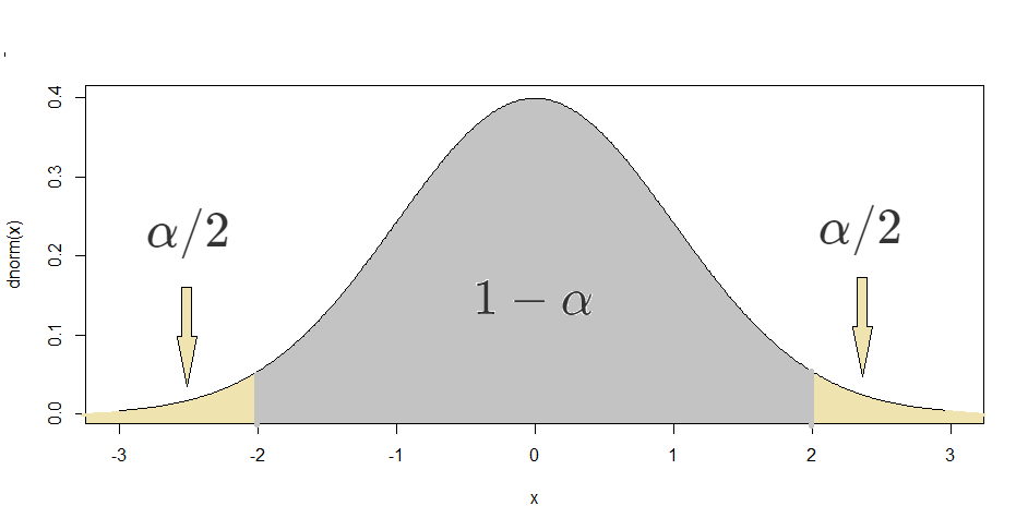
Proof. If the success-failure condition is met, the Central Limit Theorem says that \(\frac{\hat{p}-p}{\sqrt{p(1-p)/n}} \approx N(0,1).\) We can begin the construction of the confidence interval by using the symmetry of the normal PDF to find \(c\) such that \(P\left(-c\leq \frac{\hat{p}-p}{\sqrt{p(1-p)/n}}\leq c\right) = 1-\alpha.\) This is equivalent to finding \(c\) such that \(P\left(\frac{\hat{p}-p}{\sqrt{p(1-p)/n}} \leq c\right) = 1-\alpha/2\) (see figure below with the \(N(0,1)\) PDF.) Therefore, \(c\) is the inverse CDF of the standard normal distribution evaluated at \(1-\alpha/2.\) Using R’s notation, this is \(qnorm(1-\alpha/2).\) Notice that we omit the values 0 and 1 in the input of qnorm. This is because in the absence of the parameters of the normal distribution, R uses the standard normal parameters, 0 and 1. Finally, with some algebra, one can show that the statement
\[P\left(-c\leq \frac{\hat{p}-p}{\sqrt{p(1-p)/n}}\leq c\right) = 1-\alpha\] is equivalent to
\[P\left(\hat{p}-c\sqrt{\frac{p(1-p)}{n}} \leq p \leq \hat{p}+c\sqrt{\frac{p(1-p)}{n}}\right) = 1-\alpha.\]
In practice, we usually don’t have access to \(p\), so we use the estimator \(\hat{p}\) to compute the standard error \(\sqrt{\frac{p(1-p)}{n}}\) and to check the success-failure condition. That is, we check whether \(n\hat{p}\geq 10\) (number of observed successes \(\geq 10\)) and \(n(1-\hat{p})\geq 10\) (number of observed failures \(\geq 10\)).
This procedure is described in the following example.
Example 9.1 Suppose that we would like to estimate the proportion of borrowers in peer-to-peer lending programs that have a second income. We would like to provide a 95% confidence interval for such proportion, using the loans_full_schema dataset (openintro package) as a sample of borrowers. This dataset has a random sample of 10000 loans. The best estimate for the population21 proportion is the sample proportion, which is calculated as
library(tidyverse)
library(openintro)
loans <- loans_full_schema
loans |>
  count(application_type) |>
  mutate(prop = n / sum(n)) |>
  filter(application_type == "joint")
## # A tibble: 1 × 3
## application_type n prop
## <fct> <int> <dbl>
## 1 joint 1495 0.150That is, \(\hat{p}=0.1495\). Let’s check the success-failure condition for \(n=10000\) and \(\hat{p}=0.1495.\)
## [1] 1495## [1] 8505Both values are greater than 10 (by a lot), so we can use the CLT and proceed with the confidence interval computation. The critical value \(c\) is
## [1] 1.959964Therefore, the 95% CI for \(p\) is given by \[\begin{eqnarray} && \hat{p}\pm c\times \sqrt{\frac{\hat{p}(1-\hat{p})}{n}} \\ &=& 0.1495 \pm 1.96\times \sqrt{\frac{0.1495(1-0.1495)}{10000}}\\ &=& 0.1495 \pm 0.00357 = [0.1459, 0.1531]. \end{eqnarray}\]
That is, we can say that we are 95% confident that the proportion of joint applications is between 14.59% and 15.31%.
Notice that this is a very “tight” confidence interval. This is because the sample size is large enough for a high precision. If instead of 10000 we had a sample of 100 borrowers, the interval would be wider (try recalculating the interval for different values of \(n\) and different confidence levels.)
What if the success-failure condition is not met?
If the success-failure condition is not met, then one can use bootstrap simulations to find a confidence interval for \(p\), as follows.
Bootstrap sampling distribution:
library(infer)
sample_props10000 <- loans |>
  rep_sample_n(size = 10000, reps = 15000, replace = T) |>
  count(application_type) |>
  mutate(p_hat = n / sum(n)) |>
  filter(application_type == "joint")
The code above creates 15000 samples of size 10000 by sampling with replacement from the original sample. The 15000 \(\hat{p}\)s are stored in the variable sample_props10000.
We can then ask for the 0.25-quantile and 0.975-quantile of sample_props10000, which will give a 95% confidence interval for \(p\):
##   2.5%  97.5%
## 0.1426 0.1566
Confidence intervals obtained by finding the quantiles of a bootstrap sample are called percentile bootstrap confidence intervals.
9.2 Hypothesis testing for \(p\)
A hypothesis testing framework involves two complementary hypothesis, which are commonly called the null hypothesis (\(H_0\)) and the alternative hypothesis (\(H_a\)). The alternative hypothesis usually represents what we are seeking evidence for. If the data collected provides “strong” evidence in favor of the alternative hypothesis, we reject \(H_0\) in favor of \(H_a\). In the absence of such evidence, the null hypothesis is not rejected and is seen as possibly true.
A hypothesis testing procedure or hypothesis test is a rule that specifies how a sample estimate is used to make the decision to reject or not reject \(H_0\).
It is common to use p-values (probability values) and a significance level (usually denoted \(\alpha\)) to make the decision to reject or not reject \(H_0\). For example, in section 2.7, the Malaria vaccine study showed a difference in proportions (of infected individuals in the control and treatment groups) of 64.3%. We then estimated via simulation that the probability of observing a difference of at least 64.3% under the assumption that \(H_0\) was true is approximately 0.02 (2%). Considering that any probability below 5% would be “small enough” to reject \(H_0\), we then rejected \(H_0\) and concluded that there was strong evidence in favor of \(H_a\). In this example, the p-value was 0.02 and the cutoff value of 0.05 was the significance level.
Choosing a significance level for a test is important in many contexts, and a commonly used level is \(\alpha = 0.05.\) However, it is appropriate to adjust the significance level to a lower one based on the application and whether multiple tests are performed. The significance level should be determined before running the test, and not after a p-value has been calculated.
The p-value is the probability of observing data at least as favorable to the alternative hypothesis as our current data, under the assumption that the null hypothesis is true. The p-value is usually found by comparing a test statistic to the null distribution of the test statistic. The null distribution of a test statistic is the distribution of all possible values of the test statistic under the assumption that the null hypothesis is true.
In what follows, we discuss a hypothesis testing procedure that rely on the Central Limit Theorem (CLT).
Suppose that in example 9.1, we suspect that the proportion of joint applications is less than 15%. So instead of finding a confidence interval for \(p\), we could carry out a hypothesis test, with the following null and alternative hypotheses:
\(H_0\): \(p = 0.15\)
\(H_a\): \(p < 0.15,\)
where \(p\) is the (population) proportion of joint applications. For this test, we will use a significance level of \(\alpha = 0.05\).
To check the success-failure condition in a hypothesis test, we use \(p_0\) instead of \(\hat{p}\) (for a confidence interval, we use \(\hat{p}\), since there are no hypotheses):
## [1] 1500## [1] 8500Since both values are greater than 10, we pass the condition.
To perform a hypothesis test for \(p\) using the CLT, we use the following test statistic: \[Z = \frac{\hat{p} - p_0}{\sqrt{\frac{{p_0}(1-{p_0})}{n}}} \frac{0.1495-0.15}{\sqrt{\frac{0.15(1-0.15)}{10000}}} = -0.1715.\] Here \(p_0\) is the hypothesized null value (which in this example is 0.15). The denominator is the approximate standard deviation of \(\hat{p}\), which is also called the standard error of \(\hat{p}\). Under \(H_0\), when the success-failure condition is met, the distribution of \(Z\) is approximately \(N(0,1).\) That is, the null distribution of \(Z\) is a standard normal distribution. The p-value is then the probability that, under the null hypothesis, one would observe a test statistic \(Z\) at least as favorable to \(H_a\) as the one obtained from the data.
In this case, the p-value is \(P(Z < -0.1715)\), which can be computed as:
## [1] 0.4319153This means that, under \(H_0\), the probability that we would observe a \(\hat{p}\) equal to or less than 0.1495 in a sample of size 10000 is 0.43. That is, the observed \(\hat{p}\) is not unusual under \(H_0\) (since 0.43 is greater than the pre-determined significance level of 0.05). Therefore, we don’t reject \(H_0\).
Notice that in this test we were only concerned with testing one direction (whether \(p\) is less than a specific value). This type of alternative hypothesis is called a one-sided hypothesis. If we were concerned with testing whether \(p\) is different than a specific value, regardless of which direction, we would use a two-sided hypothesis. That is, \(p \neq p_0\), instead of \(p < p_0\). Two-sided alternative hypotheses are more common, and in those cases, the probability above should be multiplied by 2 to account for both tails of the distribution.
Like in the case for confidence intervals, if the success-failure condition is not met, we can use bootstrap sampling to carry out the hypothesis test. This time though, we must generate the bootstrap sampling distribution under \(H_0\) (that is, the null distribution). This can be done by specifying the probabilities for each outcome of application_type.
Bootstrap null distribution:
null_props10000 <- data.frame(application_type = c("individual", "joint")) |>
  rep_sample_n(size = 10000, reps = 15000, replace = T, prob = c(0.85, 0.15)) |>
  count(application_type) |>
  mutate(p_hat = n / sum(n)) |>
  filter(application_type == "joint")
Notice that the data is simply data.frame(application_type = c("individual", "joint")) instead of loans, and we added prob = c(0.85, 0.15) to reflect the null hypothesis.
The p-value is then calculated as the proportion of \(\hat{p}\)s that are less than or equal the observed one (0.1495):
## [1] 0.4538Notice how this p-value is close to the one calculated using the CLT. This is not a surprise since the sample is very large, so the CLT should yield a good approximation. In both cases, we do not reject \(H_0\).
9.3 Chi-square goodness-of-fit test
In the previous section, we tested whether a population proportion \(p\) could be equal to a hypothesized value \(p_0\). We would use this type of test when the variable of interest is considered to have only two outcomes: “success” (with probability \(p\)) or “failure” (with probability \(1-p\)). For variables with more than two possible outcomes, we may be interested in testing whether the probability distribution of the outcomes is consistent with a pre-determined null distribution, as demonstrated in the next example.
9.3.1 An example
Example 9.2 Consider data from a random sample of 275 jurors in a small county. Jurors identified their racial group, as shown in the figure below, and we would like to determine if these jurors are racially representative of the population. If the jury is representative of the population, then the proportions in the sample should roughly reflect the population of eligible jurors (registered voters).
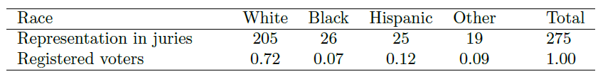
While the proportions in the juries do not precisely represent the population proportions, it is unclear whether these data provide convincing evidence that the sample is not representative. If the jurors really were randomly sampled from the registered voters, we might expect small differences due to chance. However, unusually large differences may provide convincing evidence that the juries were not representative.
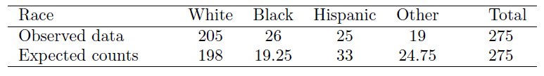
About 72% of the population is white, so in a randomly selected jury, we would expect about 72% of the jurors to be white: \(0.72\times 275 = 198\).
Similarly, we would expect about 7% of the jurors to be black, which would correspond to about \(0.07\times 275 = 19.25\) black jurors.
And so on. See the table below for the expected counts for each racial group.
We need to test whether the differences between the observed counts and the expected counts are strong enough to provide convincing evidence that the jurors are not a random sample. These ideas can be organized into hypotheses:
\(H_0\): The jurors are a random sample from the county, i.e. the racial distribution of the jurors is consistent with the racial distribution of the county.
\(H_a\): The jurors are not randomly sampled, i.e. the racial distribution of the jurors is not consistent with the racial distribution of the county.
To evaluate these hypotheses, we quantify how different the observed counts are from the expected counts. Strong evidence for the alternative hypothesis would come in the form of unusually large deviations in the groups from what would be expected based on sampling variation alone.
In the hypothesis test introduced in section 9.2, we constructed a test statistic of the following form: \[ \frac{\text{point estimate} - \text{null value}} {\text{SE of point estimate}} \] This construction was based on (1) identifying the difference between a point estimate and an expected value if the null hypothesis was true, and (2) standardizing that difference using the standard error of the point estimate. These two ideas will help in the construction of an appropriate test statistic for count data.
Our strategy will be to first compute the difference between the observed counts and the counts we would expect if the null hypothesis was true, then we will standardize the difference: \[ Z_{1} = \frac{\text{observed white count} - \text{null white count}} {\text{SE of null white count}} \] The standard error for the point estimate of the count is the square root of the count under the null22. Therefore, \(Z_1 = \frac{205 - 198}{\sqrt{198}} = 0.50.\) The fraction is very similar to previous test statistics: first compute a difference, then standardize it. These computations should also be completed for the black, Hispanic, and other groups. Here are all the computations:
White: \(Z_1 = \frac{205 - 198}{\sqrt{198}} = 0.50.\)
Black: \(Z_2 = \frac{26-19.25}{\sqrt{19.25}} = 1.54.\)
Hispanic: \(Z_3 = \frac{25-33}{\sqrt{33}} = -1.39.\)
Other: \(Z_4 = \frac{19-24.75}{\sqrt{24.75}} = -1.16.\)
We would like to use a single test statistic to determine if these four standardized differences are irregularly far from zero. That is, \(Z_1\), \(Z_2\), \(Z_3\), and \(Z_4\) must be combined somehow to help determine if they – as a group – tend to be unusually far from the hypothesized null distribution. A first thought might be to take the absolute value of these four standardized differences and add them up, but it is more common to add the squared values: \(X^2 = Z_1^2 + Z_2^2 + Z_3^2 + Z_4^2 = 5.89.\) The test statistic \(X^2\), which is the sum of the \(Z^2\) values, is called a chi-square statistic. We can also write an equation for \(X^2\) using the observed counts and null counts:
\[\begin{equation} X^2 = \frac{(\mbox{observed count}_1 - \mbox{null count}_1)^2}{\mbox{null count}_1} + \dots + \frac{(\mbox{observed count}_4 - \mbox{null count}_4)^2}{\mbox{null count}_4} \end{equation}\]
The test statistic \(X^2\) summarizes how strongly the observed counts tend to deviate from the null counts. If the null hypothesis is true, then \(X^2\) follows a new distribution called a chi-square distribution. Using this distribution, we will be able to obtain a p-value to evaluate the hypotheses.
9.3.2 Chi-square distribution
The chi-square distribution is a continuous distribution that results from the sum of squared independent standard Normal random variables. More specifically, let \(Z_1, Z_2, \dots, Z_n\) be \(n\) independent standard Normal random variables. Then the random variable \[X^2 = \sum_{i=1}^n Z_i^2\] has a chi-square distribution with \(n\) degrees of freedom. So the chi-square distribution has only one parameter, its degrees of freedom. The PDF of a chi-square distribution with \(df\) degrees of freedom is given by:
\[f(x) = \frac{e^{-\frac{x}{2}}x^{\frac{df}{2}-1}}{2^{\frac{df}{2}}\Gamma\left(\frac{df}{2}\right)}, \quad x\geq 0,\]
where \(\Gamma\) is the gamma function23.
Notation: We will use the notation \(X^2 \sim chisq(df)\) to say that \(X^2\) has a chi-square distribution with \(df\) degrees of freedom.
In R, the PDF, CDF, and inverse CDF of a chi-square distribution are the functions dchisq(x, df), pchisq(x,df), and qchisq(p, df). The chi-square distribution only takes non-negative values and it’s generally right-skewed. However, the higher its degrees of freedom, the less skewed it is, as illustrated in the figure below
library(tidyverse)
ggplot() +
  xlim(0, 15) +
  ylim(0, 0.4) +
  stat_function(aes(color = "df = 2"), fun = dchisq, args = list(df = 2)) +
  stat_function(aes(color = "df = 3"), fun = dchisq, args = list(df = 3)) +
  stat_function(aes(color = "df = 6"), fun = dchisq, args = list(df = 6)) +
  stat_function(aes(color = "df = 9"), fun = dchisq, args = list(df = 9))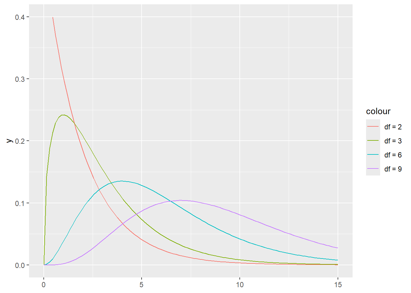
Our principal interest in the chi-square distribution is the calculation of p-values, which (as we have seen before) is related to finding the relevant area in the tail of a distribution.
Example 9.3 For a random variable that has a chi-square distribution with 5 degrees of freedom, what is the probability that its value is greater than 10?
In R, this probability can be computed as
## [1] 0.075235259.3.3 Conducting a goodness-of-fit test
Back to example 9.2, we calculated \(X^2 = Z_1^2 + Z_2^2 + Z_3^2 + Z_4^2 = 5.89\). If the sample size is “large enough”, each \(Z\) is approximately \(N(0,1)\) under the null hypothesis, and therefore \(X^2\) can be approximated by a chi-square distribution with 3 degrees of freedom. The reason we use 3 and not 4 degrees of freedom is because we only use 3 (and not 4) independent pieces of information (all four probabilities must add to 1, so once we know 3 of them, we can compute the fourth.) The traditional “large enough” condition for a chi-square goodness-of-fit test is to have at least 5 expected counts in each category under the null hypothesis. This condition is met for the jurors example. Recall that the expected counts under the null hypothesis were 198 (white), 19.25 (black), 33 (Hispanic), 24.75 (other).
Since \(X^2\) was measuring how far the observed counts were from the expected counts, we can conclude the hypothesis test by answering whether 5.89 an unusually high value for a chi-square distribution with 3 degrees of freedom. We can address this question by finding \(P(X^2 > 5.89)\) under the assumption that \(X^2 \sim chisq(3)\). This probability is the p-value for the test.
## [1] 0.1170863Under a significance level of \(\alpha = 0.05\), this p-value would not be small enough to reject the null hypothesis. Therefore, we would conclude that the juror’s racial distribution was not inconsistent with the county’s racial distribution.
Using the `chisq.test() function for a goodness-of-fit test:
To compute both the chi-square statistic \(X^2\) and the p-value for a goodness-of-fit test using R, one can use the function chisq.test(), as follows:
##
##  Chi-squared test for given probabilities
##
## data:  c(205, 26, 25, 19)
## X-squared = 5.8896, df = 3, p-value = 0.1171
Note that the first input is the vector of observed counts for each category, while the second input, p, is the vector of expected probabilities for each category (they must add to 1).
The chi-square goodness-of-fit test can summarized as follows:
Theorem 9.2 Suppose we are to evaluate whether there is convincing evidence that a set of observed counts \(O_1\), \(O_2\), …, \(O_k\) in \(k\) categories are unusually different from what might be expected under a null hypothesis. Call the expected counts that are based on the null hypothesis \(E_1\), \(E_2\), …, \(E_k\). If each expected count is at least 5 and the null hypothesis is true, then the test statistic below can be approximated by a chi-square distribution with \(k-1\) degrees of freedom:
\[\begin{equation}
X^2 = \frac{(O_1 - E_1)^2}{E_1} + \frac{(O_2 - E_2)^2}{E_2} + \cdots + \frac{(O_k - E_k)^2}{E_k}.
\end{equation}\]
The p-value for this test statistic is found by looking at the upper tail of this chi-square distribution. That is, p-value = 1 - pchisq(X2, df = k-1). We consider the upper tail because larger values of \(X^2\) would provide greater evidence against the null hypothesis.
There are two conditions that must be checked before performing a chi-square test:
- Independence. Each case that contributes a count to the table must be independent of all the other cases in the table.
- Sample size. Each particular scenario (i.e. cell count) must have at least 5 expected cases.
Failing to check conditions may affect the test’s error rates.
9.4 Confidence interval for \(p_1 - p_2\)
Sometimes we may be interested in estimating the difference between the proportions of two groups, for example, the difference in the proportion of infections between those who received a vaccine and those who didn’t (as in the malaria vaccine example in section 2.7.1). We denote the population proportions for these two groups by \(p_1\) and \(p_2\). Using \(\hat{p}_1 - \hat{p}_2\) as an estimator of \(p_1 - p_2\), we can find a confidence interval for \(p_1 - p_2\), by looking at the sampling distribution of \(\hat{p}_1 - \hat{p}_2\). The Central Limit Theorem gives the approximate sampling distribution of one sample proportion, not the difference between two sample proportions; but thankfully, we can still approximate the sampling distribution of \(\hat{p}_1 - \hat{p}_2\) by using a fact about normal distributions:
Fact: The sum of two normally distributed random variables is also normal.24
Denote by \(n_1\) and \(n_2\) the sample sizes of the two groups. The fact stated above implies that, if the success-failure condition is met for both groups, \(\hat{p}_1 - \hat{p}_2\) is approximately normal. Now we just need to find \(E(\hat{p}_1 - \hat{p}_2)\) and \(Var(\hat{p}_1 - \hat{p}_2)\) in order to find a confidence interval for \({p}_1 - {p}_2\).
\[\begin{eqnarray} E(\hat{p}_1 - \hat{p}_2) &=& E(\hat{p}_1) - E(\hat{p}_2) = {p}_1 - {p}_2.\\ Var(\hat{p}_1 - \hat{p}_2) &=& Var(\hat{p}_1) + 2 Cov(\hat{p}_1, \hat{p}_2) + (-1)^2 Var(\hat{p}_2) = \frac{p_1(1-p_1)}{n_1} + \frac{p_2(1-p_2)}{n_2}. \end{eqnarray}\]
Here we used the assumption that the data was collected independently for both groups, which implies that \(Cov(\hat{p}_1, \hat{p}_2) = 0.\)
The calculations above give us the approximate sampling distribution of \(\hat{p}_1 - \hat{p}_2\) for “large enough” samples:
\[ \hat{p}_1 - \hat{p}_2 \approx N\left(p_1-p_2, \sqrt{\frac{p_1(1-p_1)}{n_1} + \frac{p_2(1-p_2)}{n_2}}\right). \]
This gives the following result:
Theorem 9.3 (Confidence interval for the difference between two proportions) Consider a variable that takes only two possible values (0 and 1), and consider iid samples of this variable for two different groups. Then the endpoints of a \((1-\alpha)\) CI for \(p_1 - p_2\) are given by \[ \hat{p}_1 - \hat{p}_2 \pm c\times \sqrt{\frac{\hat{p}_1(1-\hat{p}_1)}{n_1} + \frac{\hat{p}_2(1-\hat{p}_2)}{n_2}}, \quad \mbox{where } c = qnorm(1-\alpha/2). \] That is, the \((1-\alpha)\) CI is: \[ \left[\hat{p}_1 - \hat{p}_2 - c\times \sqrt{\frac{\hat{p}_1(1-\hat{p}_1)}{n_1} + \frac{\hat{p}_2(1-\hat{p}_2)}{n_2}}, \hat{p}_1 - \hat{p}_2 + c\times \sqrt{\frac{\hat{p}_1(1-\hat{p}_1)}{n_1} + \frac{\hat{p}_2(1-\hat{p}_2)}{n_2}}\right]. \]
The confidence interval for \(p_1-p_2\) is a reasonable estimate if the success-failure condition is met, that is, if \(n_1p_1\geq 10\), \(n_2p_2\geq 10\), \(n_1(1-p_1)\geq 10\) and \(n_2(1-p_2)\geq 10\). Since we don’t have access to \(p_1\) and \(p_2\), we use \(\hat{p}_1\) and \(\hat{p}_2\) to check the success-failure condition. This allows us to calculate confidence intervals for the difference between two proportions, as described in the following example.
Example 9.4 Higher intake of omega-3 fatty acids has been associated with reduced risks of cardiovascular disease and cancer in some observational studies. To test whether supplementation with omega−3 fatty acids has such effects in general populations at usual risk for these conditions, a 2019 study conducted a randomized experiment among 25,871 Americans in their 50s. The group was divided into control (placebo) and treatment (omega-3) groups. The control group received vitamin D3 (at a dose of 2000 IU per day) and the treatment group received omega-3 fatty acids (at a dose of 1 g per day). Many outcomes were measured, including whether there was a major cardiovascular event at least 2 years after the study began. We wish to find a 99% confidence interval for the difference between the proportion of individuals who had a major cardiovascular event within the groups that take and don’t take omega-3. Results for this study can be found in the openintro package, under fish_oil_18. This is not a data frame, but a collection of tables with the counts for each outcome. To access the outcomes for a major cardiovascular event, we type:
##          major_cardio_event no_event
## fish_oil                386    12547
## placebo                 419    12519
So the sample proportion of individuals who had a major cardiovascular event in the treatment group was \(\hat{p}_1 = 386/(386+12547) = 386/12933 = 0.02985,\) and in the placebo group was \(\hat{p}_2 = 419/(419+12519) = 419/12938 = 0.03239.\) The denominators in these calculations are \(n_1\) and \(n_2\). The success-failure condition passes for both groups (all cell counts are greater than 10):
- \(n_1\hat{p}_1 = 386 > 10\) and \(n_1(1-\hat{p}_1) = 12547 > 10.\)
- \(n_2\hat{p}_2 = 419 > 10\) and \(n_2(1-\hat{p}_2) = 12519 > 10.\)
The critical value for a 99% CI is \(qnorm(1-0.01/2) = 2.576.\) Then the 99% CI is:
\[\begin{eqnarray} & &\hat{p}_1 - \hat{p}_2 \pm c\times \sqrt{\frac{\hat{p}_1(1-\hat{p}_1)}{n_1} + \frac{\hat{p}_2(1-\hat{p}_2)}{n_2}} \\ &=& 0.02985 - 0.03239 \pm 2.576\times \sqrt{\frac{0.02985(1-0.02985)}{12933} + \frac{0.03239(1-0.03239)}{12938}} \\ &=& -0.00254 \pm 2.576\times 0.00216 = [-0.0081, 0.003]. \end{eqnarray}\]
So we are 99% confident that the difference between the proportion of individuals who had a major cardiovascular episode within the groups who take and don’t take omega-3 is between -0.81% and 0.3%. Since 0 is within the interval, then it’s plausible that the population difference is 0. In that case, we say that there is not a statistically significant difference (at the significance level of \(\alpha=0.01\)) between the two proportions.
If the success-failure condition is not met, then one can find a confidence interval through a bootstrap simulation.
9.5 Hypothesis test for \(p_1 - p_2\)
Now let’s turn to an example of a hypothesis test for the difference between two proportions. In example 9.4, we computed a 99% confidence interval for the difference between two proportions. Alternatively, we may be interested in testing whether the two proportions are different by running a hypothesis test for the following hypotheses:
\(H_0\): \(p_1 - p_2 = 0\)
\(H_a\): \(p_1 - p_2 \neq 0.\)
The alternative hypothesis can also be one-sided (that is, “\(p_1 - p_2 > 0\)” or “\(p_1 - p_2 < 0\)”), although two-sided hypotheses are more common. We will use a significance level \(\alpha = 0.01\) for this test.
Recall that in section 9.1, we used the hypothesized null value \(p_0\) to compute the standard error of the test statistic \(Z\) and to check the success-failure condition. This is because in hypotheses tests we use the null distribution of a test statistic to compute a p-value. We shall also use the null hypothesis \(H_0: p_1 - p_2 = 0\) to compute the standard error for the difference between two proportions. However, \(H_0\) does not offer a value for \(p_1\) and \(p_2\), it only says that they are the same. Hence, we will use the same value for both proportions when computing the standard error so that we have a test statistic that better reflects the null hypothesis. We’ll call this a pooled proportion, and will call it \(\hat{p}\). The pooled proportion is calculated as the total number of successes in both groups divided by the sum of the sample sizes in both groups. In the current example, \[\hat{p} = \frac{386+419}{12933+12938} = 0.0311.\]
Now we are ready to check the success-failure condition. Recall the contingency table for this example:
##          major_cardio_event no_event
## fish_oil                386    12547
## placebo 419 12519- \(n_1\hat{p} = 386 + 419 = 805 \geq 10\) (total number of “successes”),
- \(n_2\hat{p} 12547 + 12519 = 25066 \geq 10\) (total number of “failures”).
All counts are greater than 10, so we can proceed to use the CLT.
Next we find the test statistic \(Z\) under the null hypothesis. This test statistic is similar to the one used in finding the confidence interval for \(p_1 - p_2\), but this time we use the pooled proportion \(\hat{p}\) in the calculation of the standard error, that is:
\[Z = \frac{\hat{p}_1 - \hat{p}_2}{\sqrt{\frac{\hat{p}(1-\hat{p})}{n_1} + \frac{\hat{p}(1-\hat{p})}{n_2}}} = \frac{0.02985 - 0.03239}{\sqrt{\frac{0.0311(1-0.0311)}{12933} + \frac{0.0311(1-0.0311)}{12938}}} = -1.1761.\] In R:
n1 <- 12933
n2 <- 12938
p1 <- 386/12933
p2 <- 419/12938
p <- (386 + 419)/(12933 + 12938)
Z <- (p1 - p2)/sqrt(p*(1 - p)/n1 + p*(1 - p)/n2)
Z
## [1] -1.176055The p-value is then calculated as the area of the (two) tails of the null distribution, beyond the observed \(Z\). Using pnorm:
## [1] 0.2395728Since the p-value is not smaller than the significance level \(\alpha\), we do not reject the null hypothesis, that is, we did not find strong evidence that the proportion of major cardiovascular episodes is different for those who take omega-3 and those who don’t take omega-3.
9.6 Chi-square test of independence
In the previous section, we tested hypotheses about the difference between two proportions. The sample difference was computed by through the counts of a 2-way contingency table, which summarizes the relationship between two categorical variables. The contingency table from example 9.4 involves two categorical variables with two levels. When at least one of the categorical variables has more than 2 levels, it is no longer possible to summarize the observed data as the difference between two proportions. In this case, we use a chi-square statistic to measure how far the observed proportions are from the null hypothesis. We illustrate this procedure with the following example.
Researchers recruited 219 participants in a study where they would sell a used iPod25 that was known to have frozen twice in the past. The participants were encouraged to get as much money as they could for the iPod since they would receive a 5% cut of the sale on top of $10 for participating. The researchers wanted to understand what types of questions would elicit the seller to disclose the freezing issue.
Unbeknownst to the participants who were the sellers in the study, the buyers were collaborating with the researchers to evaluate the influence of different questions on the likelihood of getting the sellers to disclose the past issues with the iPod. The scripted buyers ended with one of three questions:
- General: What can you tell me about it?
- Positive Assumption: It doesn’t have any problems, does it?
- Negative Assumption: What problems does it have?
The question is the treatment given to the sellers, and the response is whether the question prompted them to disclose the freezing issue with the iPod. The results are shown in the table below:
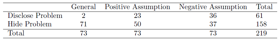
and the data suggest that asking the “negative assumption” question was the most effective at getting the seller to disclose the past freezing issues. However, you should also be asking yourself: could we see these results due to chance alone, or is this in fact evidence that some questions are more effective for getting at the truth?
The hypothesis test for the iPod experiment is really about checking whether the buyer’s question was independent of whether the seller disclosed a problem. That is, we wish to test the following hypotheses:
\(H_0:\) Disclosing the problem the type of question are independent.
\(H_a:\) Disclosing the problem the type of question are not independent.
Like with one-way tables (used in the goodness-of-fit test), we will need to compute estimated counts for each cell in a two-way table.
From the experiment,
we can compute the proportion of all sellers who disclosed
the freezing problem as \(61/219 = 0.2785\).
If there really is no difference among the questions
and 27.85% of sellers were going to disclose the freezing
problem no matter the question that was put to them,
how many of the 73 people in the General
group would we have expected to disclose the freezing
problem?
We would predict that \(0.2785\times73 = 20.33\) sellers in the General group would disclose the problem and \((1- 0.2785) \times 73 = 52.67\) to hide the problem. Obviously we didn’t observe these exact values in the data, though it is not yet clear if that is due to chance variation or whether that is because the questions vary in how effective they are at getting to the truth.
Going through the same computation for the Positive and Negative Assumption groups gives the following expected counts (in blue):
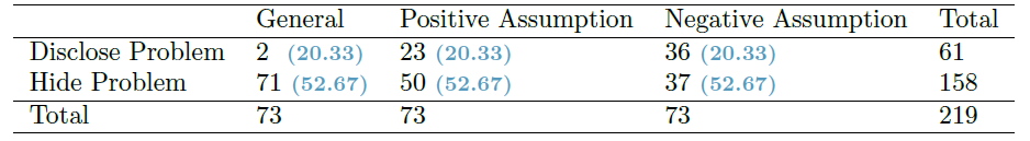
In general, expected counts for a two-way table may be computed using the row totals, column totals, and the table total. Specifically, to identify the expected count for the \(i^{th}\) row and \(j^{th}\) column, compute \[ \text{Expected Count}_{\text{row }i,\text{ col }j} = \frac{(\text{row $i$ total}) \times (\text{column $j$ total})}{\text{table total}} \]
The chi-square test statistic for a two-way table is found the same way it is found for a one-way table. We also require at least 5 expected counts in each cell to use a chi-square distribution. For each table count, compute \[\begin{eqnarray} \text{General formula}&:& \frac{(\text{observed count } - \text{expected count})^2}{\text{expected count}} \\ \text{Row 1, Col 1}&:& \frac{(2 - 20.33)^2}{20.33} = 16.53 \\ \text{Row 1, Col 2}&:& \frac{(23 - 20.33)^2}{20.33} = 0.35 \\ \vdots &:& \\ \text{Row 2, Col 3}&:& \frac{(37 - 52.67)^2}{52.67} = 4.66 \end{eqnarray}\]
Adding the computed value for each cell gives the chi-square test statistic \(X^2\): \[ X^2 = 16.53 + 0.35 + \dots + 4.66 = 40.13. \] Just like before, this test statistic follows a chi-square distribution. However, the degrees of freedom are computed a little differently for a two-way table26. For two way tables, the degrees of freedom is equal to \[ df = \text{(number of rows minus 1)}\times \text{(number of columns minus 1)} \]
In our example, the degrees of freedom parameter is \(df = (2-1)\times (3-1) = 2\). If the null hypothesis is true (i.e. the questions had no impact on the sellers in the experiment), then the test statistic \(X^2 = 40.13\) closely follows a chi-square distribution with 2 degrees of freedom. Using this information, we can compute the p-value for the test:
## [1] 1.93144e-09Using a significance level of \(\alpha=0.05\), the null hypothesis is rejected since the p-value is smaller. That is, the data provide convincing evidence that the question asked did affect a seller’s likelihood to tell the truth about problems with the iPod.
Using the `chisq.test() function for an independence test:
To compute both the chi-square statistic \(X^2\) and the p-value for an independence test using R, one can use the same function chisq.test() used for a goodness-of-fit test, but this time the input should be a contingency table, as follows:
##
##  Pearson's Chi-squared test
##
## data:  cbind(c(2, 71), c(23, 50), c(36, 37))
## X-squared = 40.128, df = 2, p-value = 1.933e-09
The function cbind() builds a table by binding columns. Here the inputs of the table were the observed counts, tallied by type of disclosure and assumption.
Keep in mind that here the target population is not the entire population of humans, but the population of borrowers in peer-to-peer lending programs.↩︎
Using some of the rules learned in earlier chapters, we might think that the standard error would be \(np(1-p)\), where \(n\) is the sample size and \(p\) is the proportion in the population. This would be correct if we were looking only at one count. However, we are computing many standardized differences and adding them together. It can be shown – though not here – that the square root of the count is a better way to standardize the count differences.↩︎
The formula for the gamma function is \(\Gamma(x) = \int_0^\infty u^{x-1}e^{-u}du.\)↩︎
The proof of this fact is not trivial and we omit it here.↩︎
An iPod is basically an iPhone without any cellular service, assuming it was one of the later generations. Earlier generations were more basic.↩︎
Recall: in the one-way table, the degrees of freedom was the number of cells minus 1.↩︎