8 Special distributions
In probability, we use the word “distribution” to refer to how all possible values of a random variable are distributed. This implies knowledge of how to calculate probabilities related to such random variable. In this chapter, we look at distributions that are encountered often in statistics and that are used to develop tools for statistical inference. More specifically, we will look at one discrete distribution (binomial) and four continuous ones (normal, t, chi-square, and F.) We describe each distribution by providing the set of all possible values of a random variable and a way to calculate probabilities for the random variable (PMF, PDF, or CDF.)
8.1 Binomial distribution
Before describing the binomial distribution, we define one of the simplest discrete random variables: the Bernoulli random variable.
A Bernoulli random variable \(X\) is an indicator random variable, that is, it only takes the values 1 (“success”) and 0 (“failure”). The probability of \(X=1\) is denoted by \(p\). Random experiments that lead to Bernoulli random variables are called Bernoulli trials. For example, the number of heads in one coin flip is a Bernoulli random variable and the coin flip is a Bernoulli trial.
A random variable \(Y\) is called a binomial random variable if it counts how many outcomes in \(n\) independent Bernoulli trials are a “success.”
Notation: We use the notation \(Y \sim Binom(n,p)\) to say that \(Y\) has the distribution of a binomial random variable with \(n\) Bernoulli trials and probability of success \(p\).
For example, the random variable \(H\) described in example 7.5 is a binomial random variable because it counts the number of heads in 2 coin flips. In this example, the Bernoulli trials are the 2 independent coin flips, and “heads” is the characteristic of interest (success). In example 7.5, it was feasible to calculate the probabilities of all possible outcomes and write the PMF. What if \(H\) was the number of heads in 20 coin flips? We could still list all possible outcomes and their probabilities, but it it turns out that there is an easy-to-use formula for the PMF of a binomial random variable.
The PMF of a binomial random variable \(Y\) is given by
\[ f(k) = P(Y = k) = {n \choose k}p^k(1-p)^{n-k}. \]
The expression \({n \choose k}\) is equal to \(\frac{n!}{k!(n-k)!}\).
The factorial of a number \(k\) is the product of \(k\) with all natural numbers less than \(k\). For example, \(4! = 4\times 3\times 2\times 1.\) It is the number of ways in which one can list \(k\) distinct objects. The factorial of 0 is 1, that is, \(0!=1\). This implies that \({n \choose 0} = {n \choose n} = 1.\)
In the formula above, \(n\) is the number of independent Bernoulli trials and \(p\) is the probability of success in each trial. The values \(n\) and \(p\) are called parameters of the binomial distribution, so when describing a binomial random variable, these values should be provided.
Example 8.1 Let \(H\) be the number of heads in 20 coin flips. Then \(H\) is a binomial random variable with \(n=20\) and \(p=0.5\). The probability of observing exactly 5 heads is
\[ P(Y = 5) = {20 \choose 5}0.5^5(1-0.5)^{20-5} = \frac{20!}{5!15!} 0.5^5 0.5^{15} = 0.01479. \]
In R, the binomial PMF is the function dbinom. More specifically, dbinom(k, n, p) = \({n \choose k}p^k(1-p)^{n-k}.\) So the probability calulation for example 8.1 can be done by running the command:
## [1] 0.01478577Example 8.2 What if we were interested in knowing the probability of obtaining at least 2 heads in 20 coin flips? In this case, we want to know \(P(H \geq 2)\). There are several ways to calculate this probability, some being unnecessarily tedious. For example, we could calculate
\[P(H\geq 2) = P(H=2)+P(H=3) + \cdots + P(H=20) = \cdots\]
or we could use the complement of \(H\geq 2\) (see section 7.1) and calculate
\[\begin{eqnarray} P(H\geq 2) &=& 1 - P(H < 2) = 1 - (P(H=0)+P(H=1)) \\ &=& 1-(1\times 0.5^0 0.5^{20} + 20\times 0.5^1 0.5^{19}) = 0.99998. \end{eqnarray}\]
R also has functions for the CDF of a random variable. For the binomial random variable \(Y\) with parameters \(n\) and \(p\), the command pbinom(k, n, p) calculates \(P(Y\leq k).\)
In example 8.2, the probability \(P(Y<2)\) can also be written as \(P(Y\leq 1)\) because \(Y\) takes only values in the natural numbers. So we can use pbinom to carry out the calculation \(P(H\geq 2) = 1 - P(H \leq 1):\)
## [1] 0.99998Notice that pbinom(1,20,0.5) returns the same value as dbinom(0,20,0.5) + dbinom(1,20,0.5).
Finally, we can also use R to plot the binomial PMF for \(H\):
x <- seq(0,20,1) # this creares a sequence that goes from 0 to 20 in steps of length 1
plot(dbinom(x, 20, 0.5) ~ x)
Changing the vaule of \(p\) to 0.1, we get:
x <- seq(0,20,1) # this creares a sequence that goes from 0 to 20 in steps of length 1
plot(dbinom(x, 20, 0.1) ~ x)
Suggestion: Try different values of \(n\) and \(p\) in the code above!
8.2 Normal distribution
A normal random variable is a continuous random variable \(X\) that takes values in the Real numbers, that is, \((-\infty, \infty)\), and has a PDF given by
\[f(x) = \frac{1}{\sigma\sqrt{2\pi}}e^{-(x-\mu)^2/{2\sigma^2}},\] for \(-\infty < x < \infty\). Here, \(\mu\) and \(\sigma\) are parameters of the normal distribution and they represent the center and spread of the distribution. More specifically, \(\mu\) is the mean of \(X\) and \(\sigma\) is the standard deviation of \(X\) (more on that in chapter 9.)
Notation: We use the notation \(X \sim N(\mu, \sigma)\) to say that \(X\) has the distribution of a normal random variable with mean \(\mu\) and standard deviation \(\sigma\). Some texbooks prefer the notation \(X \sim N(\mu, \sigma^2)\), where \(\sigma^2\) is the variance of \(X\).
A normal random variable with \(\mu=0\) and \(\sigma=1\) is called a standard normal random variable, usually denoted by \(Z\). That is, \(Z \sim N(0,1)\).
In R:
The normal PDF is the function
dnorm, whose inputs are \(x\), \(\mu\), and \(\sigma\). That is, \(dnorm(x,\mu,\sigma) = \frac{1}{\sigma\sqrt{2\pi}}e^{-(x-\mu)^2/{2\sigma^2}}.\)The normal CDF is the function
pnorm, that is, for a normal random variable \(X\sim N(\mu, \sigma)\), \(P(X\leq x) = pnorm(x, \mu, \sigma).\)For the standard normal distribution, one can omit \(\mu\) and \(\sigma\) in the functions
dnormandpnorm; in the absence of these inputs, R considers \(\mu=0\) and \(\sigma=1.\)
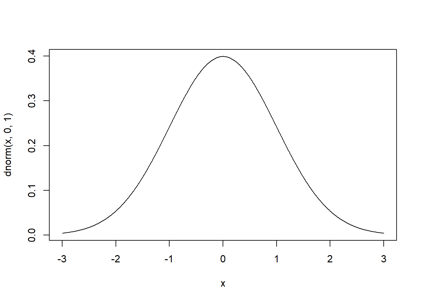
For instance, the graph of the PDF of the distribution \(N(0,1)\) is:

The input type="l" connects the points with a line. This is used for plotting continuous functions.
You have probably seen this shape before, a bell shape, which implies that values around \(\mu\) (which in this example is zero) are the most common in the normal distribution.
It turns out that any normal random variable \(X \sim N(\mu,\sigma)\) can be transformed into a standard normal variable by subtracting its mean and dividing by its standard deviation. That is, \[Z = \frac{X-\mu}{\sigma} \sim N(0,1).\]
Many variables arising from real applications are normally distributed. For example, in nature, several biological measures are normally distributed (e.g., heights, weights). The addition of several random variables also tends to be approximately normal (the Central Limit Theorem in chapter 10 speaks to this property). This implies that the normal distribution is a commonly occurring distribution in many applications.
Example 8.3 Suppose that a runner’s finishing times for 5k races are normally distributed with mean \(\mu=24.1\) minutes and standard deviation \(\sigma = 1.2\) minutes.
What’s the probability that the runner will finish her next race in less than 22 minutes?
What’s the probability that the runner will finish her next race in more than 25 minutes?
What’s the probability that the runner will finish her next race in between 22 and 24 minutes?
What’s the probability that the runner will finish her next race in exactly 24 minutes?
What should be the runner’s finishing time to ensure that its within the best 10% of her finishing times.
Answers:
Let \(X\) be the runner’s finish time in her next race. We know that \(X \sim N(24.1, 1.2).\) We use R’s pnorm for probability calculations.
\(P(X < 22) = pnorm(22, 24.1, 1.2) = 0.04.\)
\(P(X > 25) = 1 - P(X \leq 25) = 1 - pnorm(25, 24.1, 1.2) = 0.227.\)
\(P(22 < X < 24) = P(X < 24) - P(X \leq 22)\)
\(= pnorm(24, 24.1, 1.2) - pnorm(22, 24.1, 1.2) = 0.427.\)\(P(X = 24) = 0.\)
This part asks for the value of \(x\) such that \(P(X < x) = 0.10.\) That is, we need the inverse of the CDF. If we denote the CDF of \(X\) by \(F(x)\), then the answer to this question is \(F^{-1}(0.10)\). Fortunately, R also has an implementation for the inverse CDF of a normal distribution, it’s called
qnorm. So the answer to this part is \(qnorm(0.1, 24.2, 1.2) = 22.66.\) That is, the runner would need to finish her next race in less than 22.66 minutes to be within her best 10% of finish times.
Note: Keep in mind that for continuous distributions, it doesn’t matter whether we use “<” or “\(\leq\)” because the probability of one exact value occurring is 0.
The next 3 distributions are derived from the Normal distribution and arise in some sample estimates in statistics.
8.3 t distribution
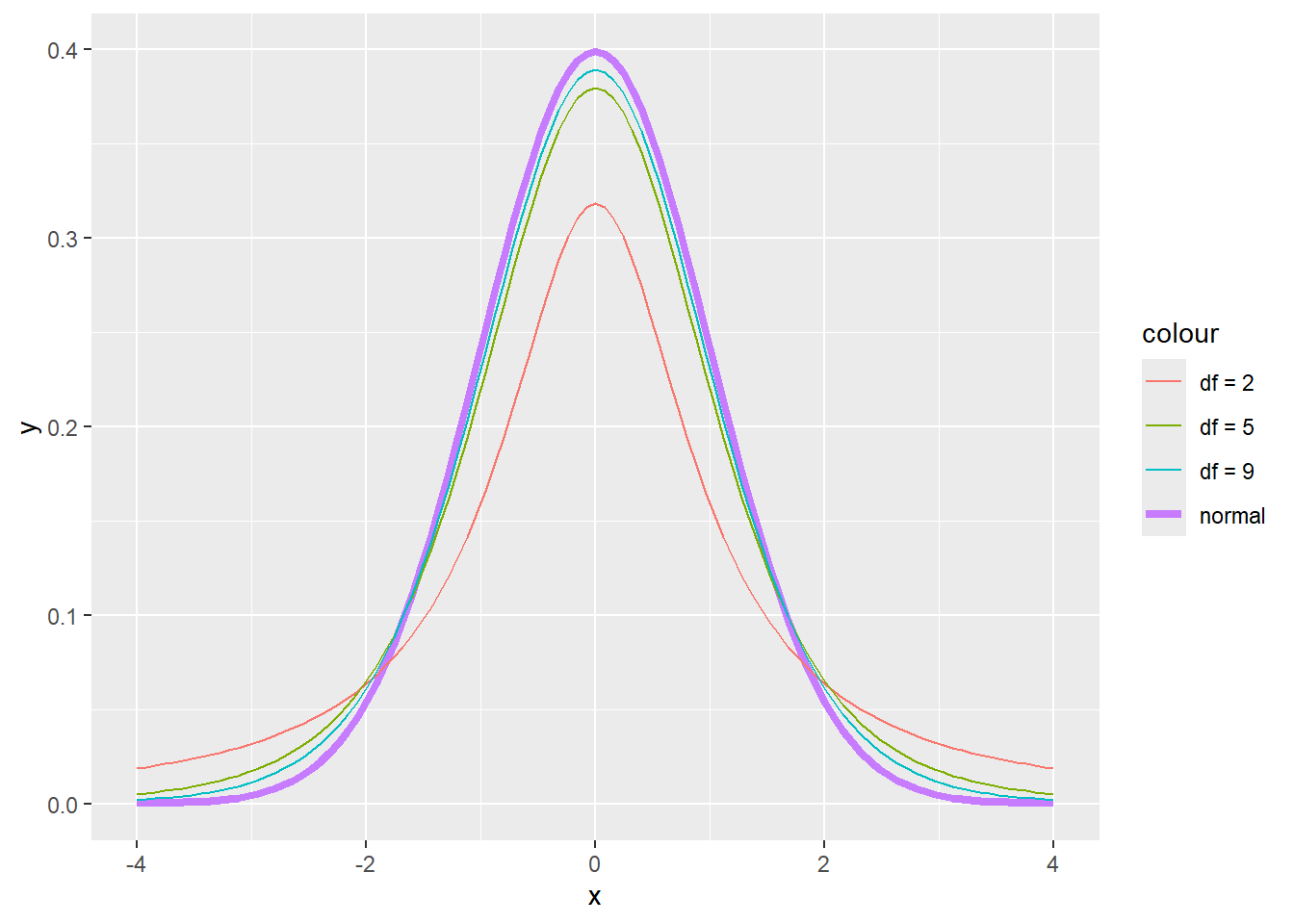
The t distribution (also known as Student’s t distribution) is a continuous distribution that resembles the standard normal one, but its PDF has thicker tails. It has only one parameter, its degrees of freedom. The PDF of a t distribution with \(df\) degrees of freedom is given by:
\[f(x) = \frac{\Gamma(\frac{df+1}{2})}{\sqrt{df\pi}\Gamma(\frac{df}{2})}\left(1+\frac{x^2}{df}\right)^{-\frac{df+1}{2}}, \quad -\infty < x < \infty,\]
where \(\Gamma\) is the gamma function19.
Notation: We use the notation \(X \sim t_{df}\) to say that \(X\) has a t distribution with \(df\) degrees of freedom.
In R, the PDF, CDF, and inverse CDF of a t-distribution are the functions dt(x, df), pt(x,df), and qt(x, df). The higher the degrees of freedom, the closer the t-distribution is to the standard Normal, as illustrated in the PDF plots below.
x <- seq(-3,3,0.01)
plot(dnorm(x,0,1) ~ x, type = "l", lwd = 2, ylab = "f(x)")
lines(dt(x, 1) ~ x, lty = 2)
lines(dt(x, 5) ~ x, lty = 3)
lines(dt(x, 10) ~ x, lty = 4)
legend("topleft", c("N(0,1)", "t(df=1)", "t(df=5)", "t(df=10)"), lty = c(1, 2, 3, 4), bty = "n")
8.4 Chi-square distribution
The chi-square distribution, also written \(\chi^2\), is a continuous distribution that results from the sum of squared independent standard Normal random variables. More specifically, let \(X_1, X_2, \dots, X_n\) be \(n\) independent standard Normal random variables. Then \[\sum_{i=1}^n X_i^2\] has a chi-square distribution with \(n\) degrees of freedom. So the chi-square distribution has only one parameter, its degrees of freedom. The PDF of a chi-square distribution with \(df\) degrees of freedom is given by:
\[f(x) = \frac{e^{-\frac{x}{2}}x^{\frac{df}{2}-1}}{2^{\frac{df}{2}}\Gamma\left(\frac{df}{2}\right)}, \quad x\geq 0,\]
where \(\Gamma\) is the gamma function (see footnote about the gamma function).
Notation: We use the notation \(X \sim \chi^2_{df}\) to say that \(X\) has a chi-square distribution with \(df\) degrees of freedom.
In R, the PDF, CDF, and inverse CDF of a chi-square distribution are the functions dchisq(x, df), pchisq(x,df), and qchisq(x, df). The chi-square distribution only takes non-negative values and it’s right-skewed. However, the higher its degrees of freedom, the less skewed it is, as illustrated in the figure below
x <- seq(0,20,0.01)
plot(dchisq(x,3) ~ x, type = "l", lty = 2, ylab = "f(x)")
lines(dchisq(x, 1) ~ x, lty = 1)
lines(dchisq(x, 5) ~ x, lty = 3)
lines(dchisq(x, 10) ~ x, lty = 4)
legend("topright", c("df=1", "df=3", "df=5", "df=10"), lty = c(1, 2, 3, 4), bty = "n")
8.5 F distribution
The F distribution is a continuous distribution that results from the quotient of 2 chi-square distributions, where each chi-square has first been divided by its degrees of freedom. More specifically, let \(X_1 \sim \chi^2_{df_1}\) and \(X_2 \sim \chi^2_{df_2}\). Then \[X = \frac{X_1/df_1}{X_2/df_2}\] has an F distribution with \(df_1\) and \(df_2\) degrees of freedom. So the F distribution has two parameters: its two degrees of freedom. The PDF of the F distribution with \(df_1\) and \(df_2\) degrees of freedom is given by:
\[f(x) = \frac{\Gamma\left(\frac{df_1+df_2}{2}\right)\left(\frac{df_1}{df_2}\right)^{\frac{df_1}{2}}x^{\frac{df_1}{2}-1}}{\Gamma\left(\frac{df_1}{2}\right)\Gamma\left(\frac{df_2}{2}\right)\left(1+\frac{df_1x}{df_2}\right)^{\frac{df_1+df_2}{2}}}, \quad x\geq 0,\]
where \(\Gamma\) is the gamma function (see footnote about the gamma function).
Notation: We use the notation \(X \sim F(df_1,df_2)\) to say that \(X\) has an F distribution with \(df_1\) and \(df_2\) degrees of freedom.
In R, the PDF, CDF, and inverse CDF of an F distribution are the functions df(x, df1, df2), pf(x,df1, df2), and qf(x, df1, df2). The F distribution only take non-negative values and it’s right-skewed. However, the higher its degrees of freedom, the less skewed it is, as illustrated in the figure below
x <- seq(0,3,0.01)
plot(df(x, 1, 1) ~ x, type = "l", ylab = "f(x)", ylim = c(0,1.2))
lines(df(x, 5, 1) ~ x, lty = 2)
lines(df(x, 10, 2) ~ x, lty = 3)
lines(df(x, 10, 10) ~ x, lty = 4)
lines(df(x, 30, 30) ~ x, lty = 5)
legend("topright", c("df1=1, df2=1", "df1=5, df2=1", "df1=10, df2=2", "df1=10, df2=10", "df1=30, df2=30"), lty = c(1, 2, 3, 4, 5), bty = "n")
The formula for the gamma function is \(\Gamma(x) = \int_0^\infty u^{x-1}e^{-u}du.\)↩︎