8 The Central Limit Theorem
The central limit theorem is the powerhouse of statistical reasoning. What we’ve done so far is largely describe data that we have. We can calculate the average based on the data we possess, or graph it in various ways, and even look at the relationship between different datas. And that’s all good, but what if we could use data that we have to understand data that we don’t have. That would be cool, huh?
Here is where we push off into the sea of inferential statistics. Inferential statistics is all about making … inferences. Inferences means drawing a conclusion based on evidence. if you come home and find the garbage can knocked over and trash spread around your floor, you might infer your dog is the culprit. You wont know, but based on all evidence that is your best guess. Similarly, we can find evidence in our data that lets us draw conclusions, not about the behavior of your dog but about the population.
We often want to know about the population, whether that is a state or a neighborhood or the country or any other body. But asking all of those people is costly and difficult. It’d be easier if we just asked a few, and were able to infer that everyone else’s answers were similar. That is the goal of inferential statistics, to infer from a sample to a population.
Why can we do that you ask? Because of the central limit theorem.
8.1 Distributions
We need to start with some different distributions though. We’ve already met a few. In charter 4 we discussed skewed distributions and the normal distributions. But distributions come in many different shapes and sizes. Let’s start by looking at what we’ve already discussed.
That’s a normal distribution, with an equal distribution above and below the mean. Another name for a normal distribution is a bell curve, because of the bell shape on creates.
In addition to normal distributions, in Chapter 4 we observed right skewed data

And data can also be left skewed.
Those three are perhaps the most typical distributions that are observed, but many others exist as well.
par(mfrow=c(1, 3))
hist(rbeta(1000, 10, 10), breaks=25, xlab="", main="Left Skewed Distribution")
hist(rbeta(1000, 30, 65), breaks=25, xlab="", main="Left Skewed Distribution")
hist(rbeta(1000, 3, 37), breaks=25, xlab="", main="Left Skewed Distribution")
Distributions come in all shapes and sizes. Data can arrange itself in many different shapes.
But here’s the important thing, the central limit theorem applies to data in any distribution, no matter what its shape is.
So what is the central limit theorem? I’ll start with the intuition of what it is, before giving the formal definition.
8.2 A Marathon Example
This example is a condensed version of the explanation of the central limit theorem in Charles Wheelan’s Naked Statsitics, which is my favorite book on stats. I tried to think of a similar explanation that would at least let me claim to be similar to, rather than a copy of what Wheelan wrote, but I couldn’t. His explanation was too clear, and any other example would muddy that.
Imagine that it’s the weekend of a big marathon in your city (think NYC marathon, but it doesn’t have to be NYC). Thousands of people from around the world have come to participate. Tour buses are provided to get runners from a sign in point to the starting line, in order to help manage the size of the crowds. However, one tour bus has gotten lost.
You’ve joined the search groups looking for this lost tour bus, full of soon-to-be marathoners. Pretty quickly you come across a broken down tour bus on the side of the street. Success! You’ve saved the day. Or have you?
You climb on the bus and notice something. All of the passengers are… larger. Not abnormally so, but they look to be overall average. It had just come up in bar trivia the night before, so you know that the average American’s woman’s weight is 168.5 ounds and that the average American man is 195.7 pounds.Some of the passengers weigh a bit more, some a bit less, but you quickly (somehow) surmise that the bus’s average weight is roughly 173 pounds.
Do you think that bus has the marathoners? It might not be impossible, but you quickly recognize that the bus you found is highly unlikely to be the one everyone is searching for. The driver confirms your suspicions, this bus had broken down on its way to a nearby amusement park.
Without knowing it you’ve applied the central limit theorem. There were thousands of runners in the city. The average marathoner’s weight will be closer to 150. Some will be larger, and some will be smaller. But that is the rough average for the population of marathoners in the city.
You an think of each tour bus, which holds about 50 runners, as an individual sample of the runners. If each tour bus was filled at random, some of the runners will be smaller than average on each bus, but some will be a bit larger, and the average of each tour bus will differ from the average of all runners somewhat. But what are the odds that one sample of runners, one tour bus, will be on average 30 pounds above average? It isn’t impossible. But it is highly unlikely.
We’re going to keep circling around a few terms, let’s make sure we’re clear:
- Population of marathoners: all marathoners in the city for the race
- Sample of marathoners: each tour bus of 50 runners
If you take a single sample of the marathoners, the average will differ slightly from the population mean. Let’s create a list of our runners, using the command rnorm(). Rnorm() generates random numbers, after we choose the number we want (n=), the mean (mean=), and the standard deviation (sd=). Once we enter that, it can output the random weight of all our runners, conforming that generally conform to that distribution.
Runners <- rnorm(n=2500, mean=150, sd=10)
hist( Runners , freq=FALSE, main="Distribution of 1500 Runner Weights")
Now we have the weights of all 1500 runners signed up for our marathon. And we want to treat each bus taking them to the start line as a sample of that population. We can take a sample of those 1500 using the command sample(). Let’s see what our first sample looks like; remember, each bus fits 50 runners.
##  [1] 153.7799 158.5400 138.8464 150.6848 165.7530 153.7104 132.9379
##  [8] 151.2301 139.9260 150.7587 131.7908 142.5554 150.9380 147.7356
## [15] 152.5600 146.1994 133.7257 155.2997 159.2586 151.7510 148.3702
## [22] 150.8102 128.8952 159.6997 161.8839 138.5345 151.6950 154.4224
## [29] 151.3097 163.1954 145.1178 154.3217 150.5398 153.0308 149.3711
## [36] 154.0341 153.6797 145.2400 133.4279 154.1151 148.5324 149.8335
## [43] 152.5648 152.4212 141.4425 144.7661 151.8582 149.0906 142.9605
## [50] 163.5343## [1] 149.3336So the mean isn’t 150. But it’s also not that far from 150 either in general. And Most wont be.
Overall, the mean of our samples, if we take enough, will equal the mean of the population. As we keep taking samples from the runners, the distribution of the means of those samples will stack up close to 150, forming a normal distribution. To illustrate, let’s take the mean weights of a bunch more tour buses. The code isn’t really worth explaining here, but I’m going to take multiple samples from the runners data, save them into a list of the samples, and figure out the mean of each sample. Then, I’ll graph those means.
runner.sample <- as.data.frame(t(replicate(50, sample(Runners, 50))))
runner.sample$mean <- rowMeans(runner.sample, na.rm=TRUE)
hist(runner.sample$mean)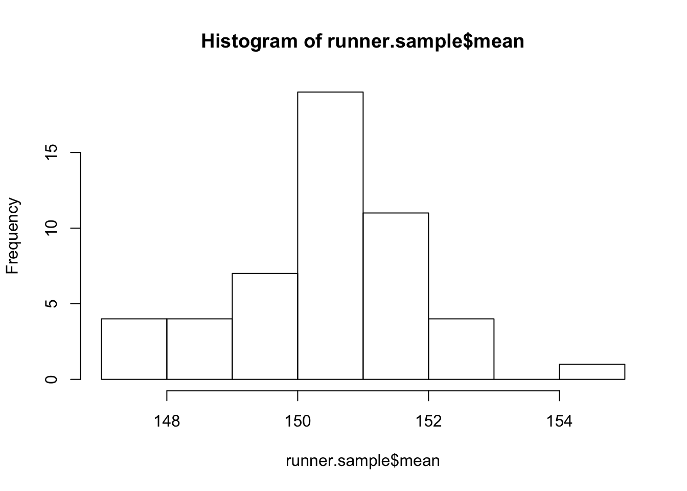
And that’s exciting, very exciting, because we know how far data should fall from the mean of a normal distribution.
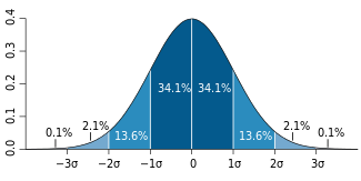
credit: Wikipedia
Remember the normal distribution. 34.1 percent of the data falls within 1 standard deviation above and below the mean. That’s on both sides, so a total of 68.2 percent of the data falls between 1 standard deviation below the mean and one standard deviation above the mean. 13.6 percent of the data is between 1 and 2 standard deviations. In total, we expect 95.4 percent of the data to be within two standard deviations, either above or below the mean.
When we’re calculating the standard deviation for the means, we divide the standard deviation for the population (10) by the square root for the sample size (50), which equals 1.41.
## [1] 1.414214Taken together, that means that if we took the mean weight of each tour bus, we would expect it to be roughly 150, and we’d expect those means to have a standard deviation of 1.41. In addition, we know that most of the data will fall within 2 standard deviations, or to be more exact between 147.42 and 152.58.
## [1] 147.18## [1] 152.82So back to the bus we located. The mean of that bus was 173. We know now that roughly 95% of the buses/samples will have a mean weight between 147.42 and 152.58. What are the odds that one bus would be at 173? Not very good. That’s 16 standard errors above the mean.
## [1] 16.31206Again, it is not impossible that the located bus is full of marathoners. What are the chances of getting a sample mean 16 standard errors above the population mean? We’ll calculate exactly ow unlikely in future chapters, but for now we can leave it at saying the chances are less than one in a million. Again, not impossible, but it is improbable.
8.3 Second Example With More Math
This is all important, so let’s work through a similar example. This example will have less of a story to it, and more of a focus on the math. But we can put it within a real world focus that might be more realistic than lost buses of runners.
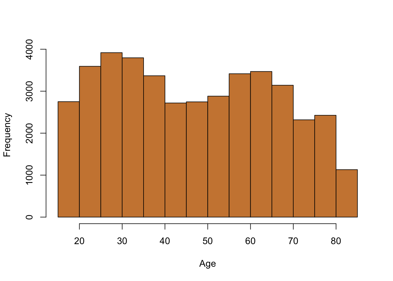
The earlier example we did above about marathoners had a normal distribution for the data on runners. However, the central limit theorem applies to any distribution of data. No matter the distribution of the original data, the means taken from random samples will become a normal distribution. So, for this example let’s use the data on California schools from earlier. The variable for the number of students per school was skewed to the right.
So, the population here is all schools in California. Let’s calculate the population mean and standard deviation.
## [1] 2628.793## [1] 3913.105The central limit theorem states that if we take repeated random samples of that population, over time the means of those samples will conform to a normal distribution. Let’s do that.
The size of each sample we take makes a small difference. Normally, you want to take a sample larger than 30 in order to accurately measure the population. But the sample can also be much larger. Let’s use 30 for this example, just to show that it works. And remember, we need to take repeated samples in order for it to form a normal distribution. Let’s start by taking 10 samples, to see the shape of those means.
student.sample <- as.data.frame(t(replicate(10, sample(CASchools$students, 30))))
student.sample$mean <- rowMeans(student.sample, na.rm=TRUE)
hist(student.sample$mean, ylim=c(0,10))
That doesn’t look very normal. Taking 10 samples isn’t enough to form a normal distribution, just like flipping a coin 10 times wasn’t in the chapter on probability. Let’s increase the number of samples to 1000 and look at the shape.
student.sample <- as.data.frame(t(replicate(1000, sample(CASchools$students, 30))))
student.sample$mean <- rowMeans(student.sample, na.rm=TRUE)
hist(student.sample$mean, breaks=100)
More normal. And 10,000 samples?
student.sample <- as.data.frame(t(replicate(10000, sample(CASchools$students, 30))))
student.sample$mean <- rowMeans(student.sample, na.rm=TRUE)
hist(student.sample$mean, breaks=100)
Fairly normal. Notice the slight outliers to the right side though. That’s because with only 30 schools in each sample, large schools are able to make those sample means larger than we’d expect. That’s fine, this distribution is what we’d expect and looks normal. So even data sampled from an extremely skewed sample can form a bell curve with enough samples drawn. What’s the standard deviation of those means? It’s the standard deviation of the population, divided by the square root of the sample size.
## [1] 714.432I keep telling you how important and exciting the existence of the central limit theorem is. In the next chapter, we’ll start using it to judge more interesting things than the destinations of tour buses. The central limit theorem underlies everything that statistics tells us about the world, for better and worse.