7 Probability
Statisticians love to talk about probabilities. Most of statistics isn’t about finding truth, so much as probable truth.
Let’s think about what we’ve discussed so far.
The median is the 50th percentile, which means half of the data is below the median and half is above (Chapter 4). That means every value has an even probability of being higher or lower than the median.
Murder and assault rates appear to be correlated (chapter 5), meaning that if you know one figure than the probability of knowing the other is increased.
But those aren’t certainties. Statistics is all about playing the odds. In this chapter we’ll review the basics of probability, which will be central to everything we do in future chapters.
7.1 Quick Definition
One quick clarification on terms. What is the difference between probabilities and odds? Odds are expressed as fractions, while probabilities are decimals. Otherwise, they are equivalent.
Let’s use rolling a die as an example. The chances of rolling a 6 are 1 out of 6. The odds of rolling a 6 are 1/6 and the probability of rolling a 6 is .1667. 1/6 equals .1667, again, because using odds or probability don’t change the chances of something occurring, just how we express them. At some point in this chapter, I will probably mess up though and say the odds are .25, but we should be clear at the start.
If we ex
7.2 Independent probabilities
We can start with one of the most basic examples of probabilities: a coin flip. What is the probability of a fair coin coming up heads? .5 or 1 out of 2 (1/2). Why? Because there are two possible outcomes (heads or tails) and heads is one of those. That’s all straight forward enough, but what is the probability of flipping heads twice in a row? The two events are independent, meaning they do not influence each other, so every possible order of flippings is equal. The coins could be heads-heads, heads-tails, tails-heads, or tails-tails. Thus, there are four possible orders, one of which is two heads, meaning the odds are 1/4 or .25.
When events are independent, you can multiple their individual probabilities to calculate their joint probabilities. With the above example, 1/2 * 1/2 = 1/4.
What are the odds of rolling two 6s in a row with fair dice? The odds of rolling one 6 is 1/6 (there are six sides to a die),so doing that twice would be 1/6 * 1/6 = 1/36.
What are the odds that you’ll get a sun burn and be robbed on the same day? Let’s estimate the odds of getting a sun burn at 1/2500 and the odds of being robbed at 1/10000 (both of which are being made up). If the chances are independent, the odds would be 1/2500 * 1/10000 which equals 1/25000000. But what happens if the reason you got a sunburn is because you fell asleep while lounging on the beach, making it easy for someone to grab your wallet? Then the odds are dependent, and we have to consider how the odds of one event impacts the probability of additional events.
7.3 Conditional Probabilities
Let’s move from dice and coins to another classic tool of teaching probability: cards. Let’ say that I have a deck of cards with all 52 cards present, and it is well shuffled. If i flip over the top card, what are the odds that it is red? Half the deck is red, so the odds would be 1/2. There is a 50-50 chance the first card is red, and a 50-50 chance it is black.
But what are the odds that the first two cards I flip over are red, and I don’t put the first card back? The odds that the first one is red is 1/2. What are the odds that the second one is red? The deck has changed. If the first one is red, now there are now only 25 red cards left (I’ve already flipped one)and there are still 26 black cards. The odds of the second card being red have now fallen, to 25/51, which is .49.
The odds for the second event were conditional on the first occurring. That isn’t true when you’re flipping a cone. The 9th coin flip is in no way affected by the 8th or the 7th or any other event. That’s an important element of independent odds and probabilities, because it allows statisticians to detect odd results.
7.4 Finding Cheaters
Let’s say your professor offers a play a game with you. They will flip a coin, and for every heads you pay them 1 dollar, and every time it shows tails you’ll get a dollar. The lesson prior they had explained that the odds of getting heads or tails was 50-50, and that the events are independent, so you know it’s unlikely that you’ll lose much money playing this game, if you lose at all, and it’ll be more fun than sitting through lecture.
The professor starts flipping the coin, and the first one is heads. They get a dollar. They flip again and heads again. They keep flipping and you keep playing because you need to make your money back, a run of tails must be coming. But no, they flip 10 more times, and 10 more heads.
Does that seem fair? You say it isn’t, but the professor insists that the events are independent. It’s absolutely possible that a coin could be flipped 12 times in a row and come up heads every time. They show how that is one possibility.
It is possible. But is it probable? You take the chalk from their hand and map out the odds. Each coin flip has a 1/2 or ,5 probability of coming up heads. The odds of two heads is .5 * .5, or .25. And you keep going, and showing that the odds of 12 heads in a row is .5 * .5 * .5 * .5 * .5 * .5 * .5 * .5 * .5 * .5 * .5 * .5. I’m going to turn it over to R to figure out what that equals.
## [1] 0.0002441406.0002. That’s roughly equivalent to 1 in 5000. It might be possible to get that many heads in a row, but you say that it is improbable. And you’re correct, it is incredibly unlikely that heads would come up that many times. It was an unfair coin, your professor was just making sure you had paid attention and returned the money.
But again, it was possible that the coin had been fair. If you flipping a fair coin a million times, there will be many streaks of 12 consecutive heads mixed in. And just because the last flip was heads does not mean that the next flip is any more likely to be tails (remember, they’re independent).
Should we expect the number of heads and tails to be 6 each if we flip a coin 12 times. Yes, and no. Yes, 6 is the most common result of 12 coin flips. But it is far from the only result.
I’ll set up a program below to flip a fair coin 12 times, and we can do it a few rounds to see what the game should have looked like.
sample.space <- c("Tails","Heads")
theta <- 0.5 # this is a fair coin
N <- 12 # we want to flip a coin 20 times

flips <- sample(sample.space,
                size = N,
                replace = TRUE,
                prob = c(theta, 1 - theta))
flips
## [1] "Heads" "Heads" "Tails" "Tails" "Tails" "Tails" "Heads" "Tails"
## [9] "Tails" "Tails" "Heads" "Heads"## [1] "Tails" "Tails" "Heads" "Heads" "Tails" "Tails" "Heads" "Heads"
## [9] "Tails" "Heads" "Heads" "Tails"## [1] "Heads" "Tails" "Heads" "Heads" "Tails" "Tails" "Tails" "Tails"
## [9] "Tails" "Heads" "Tails" "Heads"Every time I publish this book to the website that code regenerates and the set of 3 games is replayed. That means I can’t tell you the result. How many times does the professor win, and how many times does the student? I am guessing that it wasn’t 6 heads and 6 tails though all 3 times regardless.
That’s because the probabilities of getting a certain number o heads or tails follows a well established distribution. If we play the game of 12 flips thousands of times, the largest number will be a 6-6 outcome. But every other outcome 7-5, 5-7, 8-4, etc., will occur too. Let’s plot that distribution below, as if we played the game 5000 times. The x-axis will show the number of heads observed in each game, while the y-axis shows the number of games that outcome was reached out of 5000.
##    count result
## 1      0      4
## 2      1     14
## 3      2     82
## 4      3    266
## 5      4    644
## 6      5    932
## 7      6   1152
## 8      7    938
## 9      8    596
## 10     9    257
## 11    10     96
## 12    11     18
## 13    12      1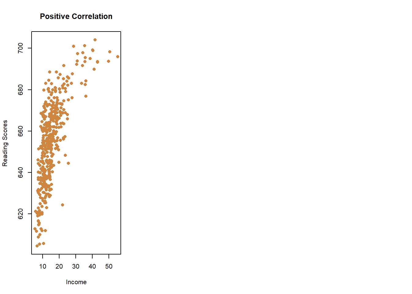
Look at that, 1 time out of the 5000 12 heads did come up in a row, although 12 tails came up 4 times. However, although 12 heads did happen we know that it’s unlikely because it happened so few times out of 5000. It was possible that you were that unlucky, but a simpler explanation was that the professor was cheating.
These types of tests for cheating show up in the real world. A few years back school officials started to think that there might be widespread cheating on standardized tests in Atlanta, Georgia. And not by the students, but by the teachers. Standardized tests were being used to hold teachers accountable, so they had incentives to make sure that their students did well. Why would they think there was cheating going on? Were the teachers working with the class while the test was taken, or handing out answer sheets?
It was because of the pattern of erasing on scantrons. When an answer is erased, there’s a probability that the new answer is correct or wrong. But what if you noticed that all of the answers that were erased were correct, would that seem suspicious? Not one or two answers, but hundreds. And what if all of the students in the same class erased the same answers, getting them all correct? Again, it’s possible that such a thing could happen by chance. But it was improbable.
The teachers had been changing the answers after the test was taken, but before they were submitted. They weren’t caught by a fellow teacher or someone seeing them do the erasing. They were caught by statistics and probability.
7.5 Law of Large Numbers
What if we had played the game fewer times? The distribution of heads will change it’s appearance slightly, depending on how many times we play. Imagine that I’m just going to stay in class all day flipping coins in rounds of 12, playing with anyone that’s willing to play with me. If I played 10 rounds one day, what would the outcomes might be?
##    count result
## 1      0      0
## 2      1      0
## 3      2      0
## 4      3      1
## 5      4      1
## 6      5      4
## 7      6      1
## 8      7      2
## 9      8      1
## 10     9      0
## 11    10      0
## 12    11      0
## 13    12      0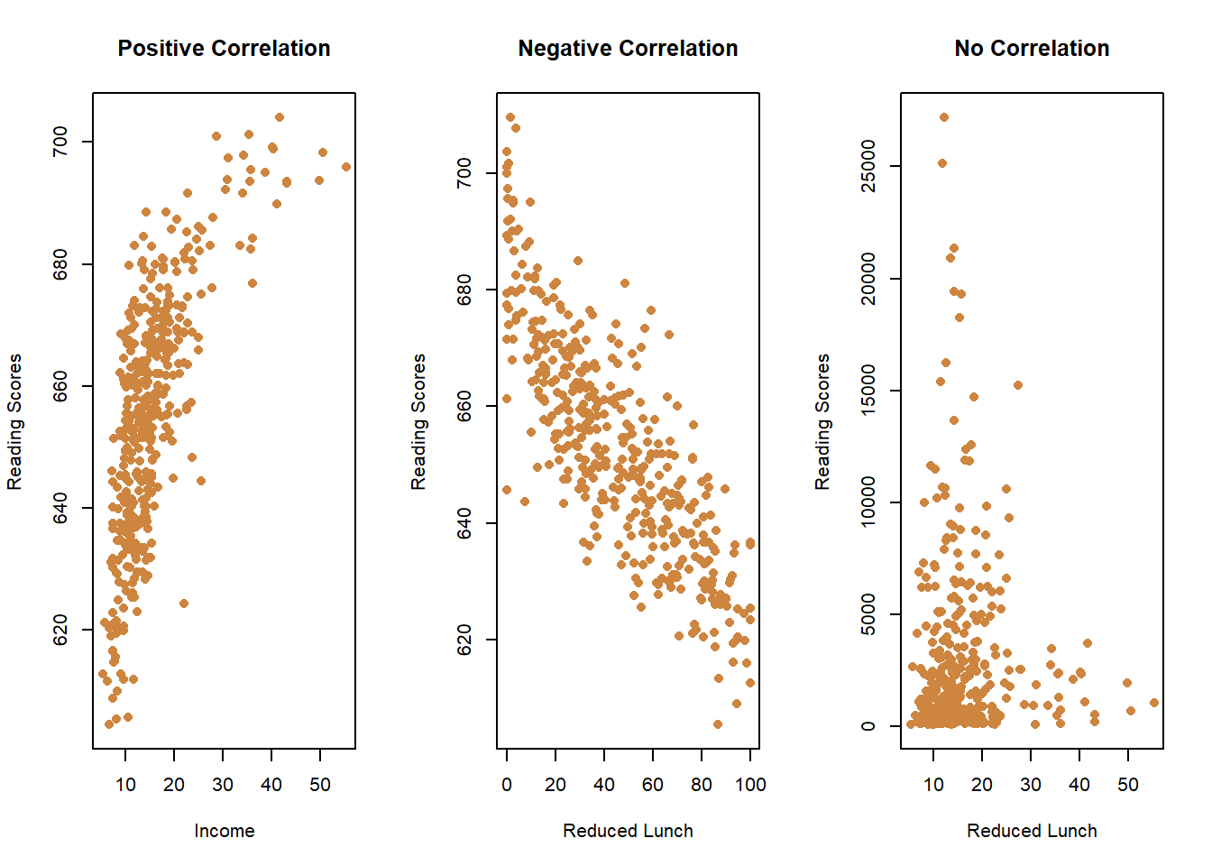
That looks different than earlier. The most common result was 5, not 6. The results still cluster towards the middle, though unevenly. Overall, I would have lost money over the day, because 6 times more tails came up than heads.
Imagine if if word gets out though and lots more student start coming by the classroom hoping to play, having heard they can win easy money? The next day 100 games with 12 flips each are played.
##    count result
## 1      0      0
## 2      1      0
## 3      2      1
## 4      3     14
## 5      4     13
## 6      5     22
## 7      6     17
## 8      7     15
## 9      8     13
## 10     9      2
## 11    10      3
## 12    11      0
## 13    12      0
The second day I lost 50 games, tied 17, and only won 33. Word is really getting out now. The next day I somehow play 10000 games (This is now a full time job).
##    count result
## 1      0      3
## 2      1     30
## 3      2    142
## 4      3    530
## 5      4   1212
## 6      5   1985
## 7      6   2240
## 8      7   1969
## 9      8   1156
## 10     9    533
## 11    10    164
## 12    11     31
## 13    12      5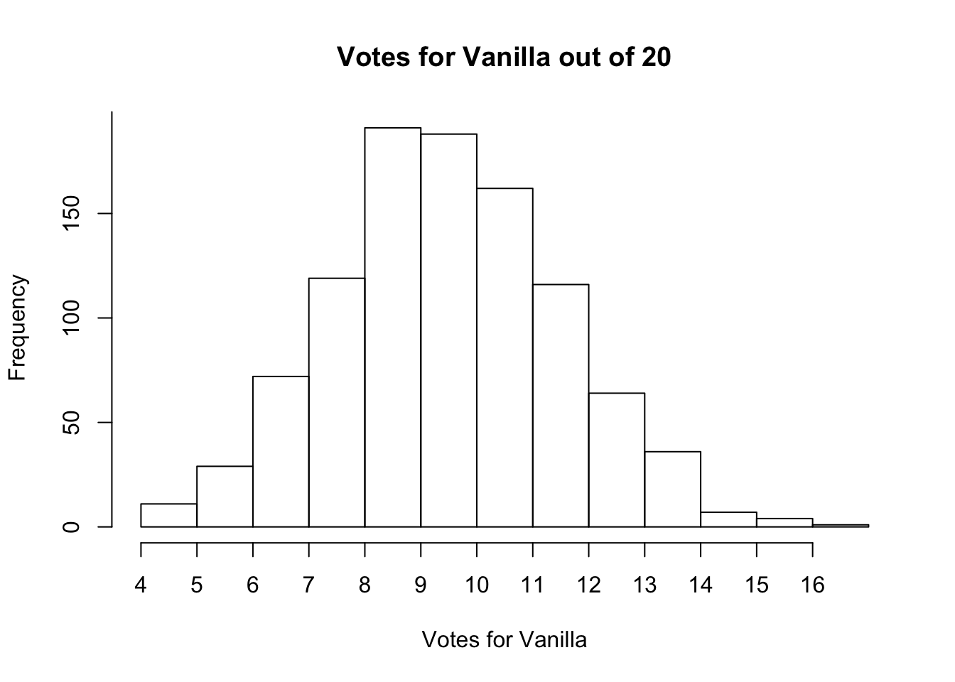
Look back to the game with 10 rounds to compare against this one. The more we play, the more symmetrical the data becomes. In the long run, if I keep playing, the game will break even for me - some rounds I win, some rounds I lose, but playing 10000 is very unlikely to mean I lose 10000 dollars, its far more likely I’ll end up losing 0. The law of small numbers means that any one game can mean a victory or defeat, but the law of large numbers means that in the long run probabilities will even out.
7.6 Expected Value
So should you have played the game in the first place? It doesn’t really matter because the expected value was 0 dollars. Let me explain.
Each game was being played for 1 dollar. You had a .5 probability of winning each round (or thought you did), but also a .5 chance of losing. So you had a .5 chance of winning 1 dollar (+1) and the same for losing (-1). What you do is multiply the payout for winning by the odds of winning, and add that to the losses from losing and the odds of losing
## [1] 0They cancel each other out. We can get more complex with the game too. If we played only twice there are four outcomes: both heads, both tails, heads-tails, and tails-heads. The odds of two heads is .25, which would mean a lose of 2 dollars. Two tails, with odds of 25, would mean you won 2 dollars. And either split would mean 0 dollars.
## [1] 0Sometimes one of us would win a few dollars, but in the long run we’d end up even and just pass dollars back and forth. That’s why I say it doesn’t really matter if you play.
What if I really want to play, so I offer you 2 dollars if you win, but you still have to only pay me 1 if I win? You should play that game (if you can afford to lose a dollar). Why? You have positive expected value.
## [1] 0.5You wouldn’t win every round, but play long enough and your higher rates of return will add up. Should you offer to pay me 2 dollars if you’ll only win 1? Probably not, unless you want to lose money in the long run.
## [1] -0.5That might all seem trivial, but it’s the exact science that Vegas has mastered. Take roulette. There are 37 numbers on a roulette wheel, so your chance of being right is 1 in 37. But casinos will only pay you with 35 times your bet. So if you bet 1 dollar, your expected value looks like this:
## [1] -0.001544402That’s a small amount, but Vegas is there to play all day to collect those fractions of pennies. Sometimes you’ll win, maybe on your first try. And when you do you will have more money than when you started, and you should walk away. But if you played 5000 times, you would certainly lose in the long run. Probabilities are what built Vegas.
Probabilities are also what built insurance agencies.
What if a company offers you a 50 dollar insurance plan on your 500 dollar smartphone? That might be a good deal, depending on the odds that your phone has an issue. Should you get the plan if there’s only a 5 percent (.05) chance that your phone breaks? We can put that in the same terms of winning and losing as above. If you buy the insurance, you’re making a 50 dollar bet that your phone will break, and that you’ll get a new phone for only 50 dollars, you’d essentially win 450 dollars (500 minus the cost of insurance). However, if your phone doesn’t break, you’re out 50 dollars (-50). And remember, there is a .05 probability that your phone will break at some point.
| Breaks | No Break | |
|---|---|---|
| With Insurance | 450 * (.05) | -50 * (1-.05) |
## [1] -25Your expected value of the insurance plan would be -25 dollars. There odds of your phone breaking are too low to justify the costs of the plan. What if the plan still cost 50 dollars, but the odds of the phone breaking were 20 percent (.20)
## [1] 50Now you have surplus value. The lesson here is that in evaluating probabilities, you have to take into account both the costs associated and the odds of an event occurring. Your cell phone company is probably going to make sure that the expected value is higher on their end (the first scenario). Why? Because like Vegas, they want to make money in the long run. They know that everyone’s phone wont break. In fact, if the probability of your phone breaking is .05, that means 1 in 20 peoples phones will break. They need to take money from the other 19 people, in order for it to make sense for them to pay for that one unlucky persons new phone. That’s the whole concept underlying insurance pools.
It wouldn’t really make sense for them to make the expected value 0, because how would they stay in business? And it might still make sense for you to buy insurance. If you can’t afford to get a new phone for 500 dollars, it probably makes more sense to get the insurance to ensure that yours wont be lost. Your expected value from health and car insurance are probably negative, but the costs of a new car or arm are so high that you can’t afford it when you’re the unlucky person to lose a bet. For insurers, some weeks more phones will break, and some weeks fewer will, but for insurers that evens out in the long run because they’re assuming that like coin flips each event is independent. Imagine if they weren’t, and 20 unlucky events happened to all 20 people with insurance on their phone the same day. What would the insurer have to pay in order to replace all those phones? They’d be our 500 dollars to 20 people, or:
## [1] 10000And they only collected 50 dollars for each contract:
## [1] 1000That’s a big lose. And maybe there could be one day that unlucky (like the 12 heads in a row) but most days will be far more normal because phone’s breaking are independent events.
What if you’re offering insurance in something that isn’t independent? Imagine that you live in New Orleans, but you’re traveling at the moment in Europe. Your mother calls you to say that they’re watching the national news and your neighbor is being interviewed about being rescued from their flooded house. Do you think the probability that your house has flooded are still the same, or did they just increase in your mind? They’ve probably gone up, because floods have conditional probabilities. If the probability of flooding in any year is .01, knowing that your neighbor was flooded probably increase yours ten fold.
7.7 False Positives
So far we’ve only talked about things that happen, such as a coin being flipped (heads or tails). You flip the coin, there’s a 50-50 chance, and one outcome comes up. We often think of probabilities as only have two outcomes, but that’s often not true, particularly with tests. Imagine you’re a woman over 40 so you go in to the doctor for a routine breast exam. 1 in 100 women have breast cancer at 50, which gives you a probability of having the disease of .01. That’s a low chance, so you start the day in a good mood. But the results come back, and you’ve tested positive. That’s bad news, probably. What are the odds that you don’t have breast cancer though? Doctors would actually struggle with that question, as shown by Gerd Gigerenzer, who tested the math literacy of medical doctors. He gave doctors a situation similar to the one described above, and three more helpful facts:
- The probability that a 50-year-old woman has breast cancer is 1% (“prevalence”)
- If a woman has breast cancer, the probability that she tests positive is 90% (“sensitivity”)
- If a woman does not have breast cancer, the probability that she nevertheless tests positive is 9% (“false alarm rate”)
He gave the doctors three options, for the probability that the woman actually has cancer
A. 9 in 10 B. 8 in 10 C. 1 in 10 D. 1 in 100
Half thought the odds were nine in ten; the correct answer was much lower, only 1 in 10. Ironically, fewer got the answer correct that random probability would have predicted.
How can the chances be so low?
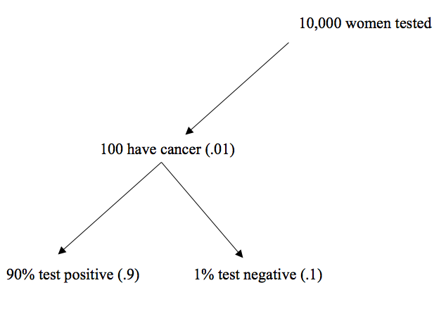
Let’s say that we open a new clinic in a city and offer free tests for breast cancer. In this example we’ll have to pretend that every woman has a 1 percent chance of having barest cancer, which isn’t true but it sure helps the math.
We get 10000 customers our first month So of those 10000 women, how many have breast cancer? With a probability of .01, we get
## [1] 100100 women of our 10000 have breast cancer. Our test is 90% accurate, meaning that of those 100 women 90 will get a positive result, but the other 10 percent will get an inaccurate negative result.
## [1] 90## [1] 10That’s one branch of the probability tree we’re developing, let’s picture it below
Great, we’ve provided accurate information to 90 women and can help them seek treatment. These are true positives. Unfortunately, the test didn’t catch the cancer in the 10 other women, so it’ll be important to communicate to them the odds that they still have cancer despite the negative test.Those are considered false negatives, because the test was negative and inaccurate.
But they aren’t the people tested that are at risk. What about the 9900 women who don’t have cancer? Well the test is only 90 percent accurate. Since 9900 women don’t have cancer, we know that 90 percent will get correct negative results.
## [1] 8910These are true negatives. 8910 women will be told they don’t have cancer, and it will be correct. What about the others?
## [1] 990Those are the false positives. 990 women will be told they have cancer, despite not having it. For them, it may set off additional and more invasive testing or the possibility of prematurely starting treatment. Here is the complete probability tree.
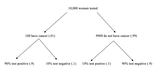
Back to our original question, what were the odds that a 50 year old women that tested positive did have cancer? Essentially, we need to figure out what are the odds that someone who has a positive test is among those that actually have cancer.
The number with a positive test is 1080, because 90 did from the left side of the figure and 890 did on the right. The number that had a positive test and cancer was 90. So, the odds are 90 (positive test AND cancer) divided by 1080 (positive test)
## [1] 0.08333333Roughly, one in ten. That’s a lot of false positives. What is the risk of a false negative? If someone immediately goes in for surgery for a disease they don’t have, their risk of an infection or other complications have greatly increased. Such concerns have led health officials to seek more accurate ways to test for diseases (reduce false positives and false negatives) and reconsider recommendations on regularized tests.
7.8 Probabilities and Correlations
We started this chapter by talking about how correlations and probabilities are useful together, in thinking about how the probability of a state have a higher murder rate increases if you know they have a high assault rate.
Companies have figured this out with their recommendations and targeted ads. What are the chances that you will buy a dog bed soon? They’re pretty low for everyone, but are much higher for someone that just started looking at books about training puppies on Amazon. There’s a correlation between the two purchases and a conditional probability, so the expected value of showing you an ad for dog beds goes up based on your search history. As you search for other things, the expected value of other ads shifts, but Amazon will continue to play the odds for the long run by showing you the best ads they can, forever. I can’t explain how they know to show you searches for things you’ve only thought about looking for though, that’s just creepy. But however they do it, it probably relies on statistics.