9 Hypothesis Testing
In this chaper we’ll start to use the central limit theorem to its full potential.
Let’s quickly remind ourselves. The central limit theorem states that for any population, the means of repeatedly taken samples will approximate the population mean. Because of that, we could tell a bus of lost individuals was very very unlikely to be headed to a marathon. But we can do more, or at least we can answer quetions that come up in the real world.
Most importantely, what we can do with a knowledge of probabilities and the central limit theorem is test hypotheses. I believe this is one of the most difficult sections to understand in an intro to statistics or research methods class. It’s where we make a leap from doing math on known things (how many inches is this loaf of bread?) to the unknown (Is the baker cheating customers?)
9.1 Building Hypotheses
A hypothesis is a statement of a potential relationship, that has not yet been proven. Hypothesis testing, the topic of this chapter, is a more formalied version of testing hypotheses using statistical tests. There are other ways of testing hypothesis (if you think a squirrel is stealing food from a bird feeder, you might watch it to test that hypothesis), but we’ll focus just on the methods statistics gives us.
We use hypothesis testing as a structure in order to analyze whether relationships exist between different pheonomena or varaibles. Is there a relationship between eating breakfast as a child and height? Is there a relationship between driving and dementia? Is there a relationship between misspellings of the word pterodactyl and the release of new Jurassic Park movies? Those are all relationships we can test with the structure of hypothesis testing.
Hypothesis testing is a lot like detective work in a way (or at least the way criminal justics is supposed to be managed). What is the presumption we begin with in the legal system? Everyone is presumed innocent, until they are proven beyond a reasonable doubt to be guilty. In the context of statistics, we would call the presumption of innocence the null hypothesis. That term will be important, the null hypothesis states what our begining state of knowledge is, which is that there is no relationship between two things. Until we know a person is un-innocent,they are innocent. Untill we know there is a relationship, there is no relationship. It is generally written as H0, H for hypothesis and 0 as the starting point.
H0: The defendent is innocent.
Should our tests and evidence not disprove the null hypothesis, it will stand. We must provide evidence to disprove it. Thus, it is the prosecutors or researchers job to prove the alternative hypothesis they have proposed. We can have multiple alternative hypothesis, and we generally write them as H1, H2, and so on.
H1: The defendent committed the crime.
I should say something more about null hypotheses. Because it is the starting point of the tests, we generally aren’t concerned with proving it to be correct. As Ronald Fisher, one of the people that developed this line of statistics said, a null hypothesis, is “never proved or established, but is possibly disproved, in the course of experimentation”. It doesn’t matter if the defense attorney proves that the defendent is innocent. It can help, but that isn’t what’s important. What matters is whether the prosecutor proves the guilt. The jury can walk away with questions and be uncertain, they may even think there’s a better than 50-50 chance the accused commited the crime, but unless guilt is proven beyond a resonable doubt they are supposed to find them innocent. Our hypothesis tests works the same way.
Unless we prove that our alternative hypothesis (H1) is correct beyond a reasonable doubt, we can not reject the null hypothesis (H0). That phrase may sound slightly clunky, but it’s specific to the context of what we’re doing. We are attempting with our statistical tests to reject the null hypothesis of no relationship. If we don’t, we say that we have failed to reject the null.
One more time, because this point that will come up on a test at some point. We are attempting to disprove the null hypothesis, in order to confirm the alternative that we have proposed. If we do not, we have failed to reject the null - not proven the null, failed to reject the null.
9.1.1 An Example
What might that look like in a social science context?
Let’s say your statistics professor is always looking for ways to boost their students learning. They hypothesize that listening to classical music during lectures will help students retain the information. How could they measure that? For one thing, they could compare the grades of students that sit in class with classical music playing, against those that don’t. So to be more specific, the hypothesis would be that listening to classical music increases grades in intro to stats classes.
So what is the null hypothesis in that case, or stated differently, what is the equivalence of innocence, in the case of classical music and grades? The null hypothesis that needs to be disproven is that there is no effect of classical music.
H0: CLassical music has no effect on student grades.
And what we want to test with our hypothesis is that classical music does have an effect.
H1: Classical music improves student grades.
The professor could collect data on tests taken by one class where they played classical music and another where they didn’t If they compared the grades, they may be able to reject the null hypothesis, or they may fail. In the next section we’ll describe a bit more about what that looks like.
9.2 Rock The Hypothesis
In 2004, researchers wanted to test the impact of tv commercials that would encourage young voters to go to cast votes. In order to test the impact of tv commercials, they chose 43 tv markets (similar to cities, but slightly larger) that would see the commercials several times a day, and selected other similar tv markets that wouldn’t see the commercial. That way, they could observe whether watching the commercial had any impact on the number of 18 and 19 year olds that actually voted in the 2004 Presidential Election.
H0: TV commercials had no impact on voting rates by 18 an 19 year olds H1: TV commercials increased voting rates by 18 an 19 year olds
The data from their test is avaliable in R with the pscl package and the dataset RockTheVote.
Before we start, we should make sure we understand the data we are using. We can us nrow() to see how many observations are in the data.
## NULLTHere are 85 tv markets that are studied. Next we can look at the summary statistics to get an idea of the varaibles available.
| strata | treated | r | n |
|---|---|---|---|
| Min. : 1.00 | Min. :0.0000 | Min. : 21.0 | Min. : 30.0 |
| 1st Qu.:10.00 | 1st Qu.:0.0000 | 1st Qu.: 83.0 | 1st Qu.:159.0 |
| Median :20.00 | Median :0.0000 | Median :109.0 | Median :226.0 |
| Mean :20.02 | Mean :0.4941 | Mean :151.1 | Mean :280.8 |
| 3rd Qu.:30.00 | 3rd Qu.:1.0000 | 3rd Qu.:194.0 | 3rd Qu.:370.0 |
| Max. :40.00 | Max. :1.0000 | Max. :718.0 | Max. :990.0 |
| p | treatedIndex |
|---|---|
| Min. :0.2570 | Min. : 1.00 |
| 1st Qu.:0.4752 | 1st Qu.:10.00 |
| Median :0.5324 | Median :21.00 |
| Mean :0.5304 | Mean :20.87 |
| 3rd Qu.:0.5946 | 3rd Qu.:31.00 |
| Max. :0.7804 | Max. :42.00 |
Treated is a dichotomous numerical varaible, that is 1 if the tv market watched the commercials, and is 0 if not. The mean here indicates that 49.41% of the tv markets were treated, and the remainders were untreated. In an experiment, researchers create a treatment group (those that saw the commercials) and a control group, in order to test for a difference.
r is the number of 18 and 19 year olds that voted in the 2004 election. The average tv market had 151 young registered voters that cast votes in the election.
n is the number of registered voters between the ages of 18 and 19 in each tv market.
p is the percentage of registered voters between the ages of 18 and 19 that voted in the election, meaning it could be calcualted by dividing r by n.
Strata and treatedIndex aren’t important for this exercise. The different tv markets were chosen because they were similar, so there is one market that saw the commercaisl and another similar market that didn’t. The varaible strata indicates which markets are matched together. treatedIndex indicates how many treated tv markets are above each observation. Full confession, I don’t totally understand what treatedIndex is supposed to be used for.
So to restate our hypotheses, we intend to test whether being in a tv market that saw commercails encouraging young adults to vote (treated) incaresed the voting rates among 18 and 19 year olds (p). The null hypothesis which we are attempting to reject is that there is no relationship between treated and p.
So what do we need to do to test the hypothesis that these tv commercials increased voting rates?
Last chapter we saw how similar the mean of the tour bus we found was to mean of the population of marathoners. Here, we don’t know what the population of 18 and 19 year old voters is. But we do have a control group, which we assume stands in for all 18 and 19 year olds. We’re assuming that the treated group is a random sample of the population of 18 and 19 year olds, so they should have the same exact voting rates as all other 18 and 19 year olds. However, they saw the commercials, so if there is a difference between the two groups, we can ascribe it to the commercials. Thus, we can test whether the mean voting rate among the tv markets that were treated with the commercials differs sigificantly.
Let’s start then by calculating the mean voting rate for the two groups, the treated tv markets and the control group. We can do that by using the subset() command to split RockTheVote into two data frames, based on whether the tv market was in the treated group or not.
treatment <- subset(RockTheVote, treated==1)
control <- subset(RockTheVote, treated==0)
mean(treatment$p)
## [1] 0.5451407## [1] 0.5160555The average voting rate among 18 and 19 year olds for the tv markets that saw the commercials is .545 or 54.5%, and the averge for the tv markets that were not treated is .516 or 51.6%. Interesting, the mean differs between the two samples.
However, as we learned last chapter, we should expet some variation between the means as we’re taking diferent samples. The means of samples will conform to a normal distribution over time, but we should expect varaiation for each individual mean. The question then is whether the mean of the treatment group differs significantly from the mean of the control group.
9.2.1 Statistical Significance
Statistical significance is important. Much of social science is driven by statistical significance. We’ll talk about the limitations later, for now though we can describe what we mean by that term. As we’ve discussed, the means of samples will differ from the mean of the population somewhat, and those means will differ by some number of standard deviations. We expect the majority of the data to fall within two standard deviations above or below the mean, and that very few will fall further away.
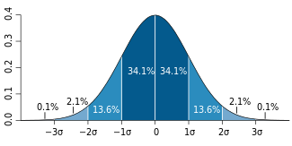
credit: Wikipedia
34.1 percent of the data falls within 1 standard deviation above and below the mean. That’s on both sides, so a total of 68.2 percent of the data falls between 1 standard deviation below the mean and one standard deviation above the mean. 13.6 percent of the data is between 1 and 2 standard deviations. In total, we expect 95.4 percent of the data to be within two standard deviations, either above or below the mean. - The Professor, one chapter earlier
That means, to state it a different way, that the probability that the mean of a sample taken from a population being within 2 standard deviations is .954, and the probability that it will fall further from the mean is only .046. That is fairly unlikely. So if the mean of the treatment group falls more than 2 standard deviations from the mean of the control group, that indicates it’s either a weird sample OR it isn’t from the same population. That’s what we concluded about the tour bus we found, it wasn’t drawn from the population of marathoners. And if the tv markets that saw the commercaials are that different from the markets that didn’t watch, we can conclued that they are different because of the commercials. The commercials had such a large effect on voting rates, they have changed voters.
So we know the means for the two groups, and we know they differ somewhat How do we test them to see if they come from the same poplation?
9.3 T-Test
The easiest way is with what’s called a t-test, which quickly analyzes the means of two groups and determines how many standard deviations they are apart. A t-test can be used to test whether a sample comes from a certain population (marathoners, buses) or if two samples differ significantly. More often than not, you will use them to test whether two samples are different, generally with the goal of understanding whether some policy or intervention or trait makes two samples different - and the hope is to ascribe that difference to what we’re testing.
Essentially, a t-test does the work for us. Interpretting it correctly then becomes all the more important, but implementing it is straight forward with the command t.test(). Within the parentheses, we enter the two data frames and the varaible of interest. Here our two data frames are named treatment and control and the variable of interest is p
| Test statistic | df | P value | Alternative hypothesis | mean of x | mean of y |
|---|---|---|---|---|---|
| 1.354 | 83 | 0.1794 | two.sided | 0.5451 | 0.5161 |
We can slowely look over the output, and discuss each term that’s produced. These will help to clarify the nuts and bolts of a t-test further.
Let’s start with the headline takeaway. We want to test whether tv commercials encouraging young adults to vote would actually make them vote in higher numbers. We see the two means that we calucalted above. 54.5% of registered 18 and 19 year olds in communities where the commercials were shown vote, while in other tv markets only 51.6% did so. Is that significant?
The answer to that quesiton is shown below P value, and the result is no. We aren’t very sure that these two groups are different, even though there is a gap between the means. We think that difference might have just been produced by chance, or the luck of the draw in creating different samples. The p value indicates the chances that we could have generated the difference between the means by chance: .1794, or roughly .18 (18%), and we aren’t willing to declare something different if we’re only 18% sure they’re different.
Why are we that uncertain? Because the test statistic isn’t very big, which helps to indicate the distance betwene our two means. The formula for calculating a test statistic is complicated, but we will discuss it. It’s a bit like your mother letting you see everything she has to do to put together thanksgiving dinner, so that you learn not to complain. We’ll see what R just did for us, so that we can more fully apprecaite how nice the software is to us.
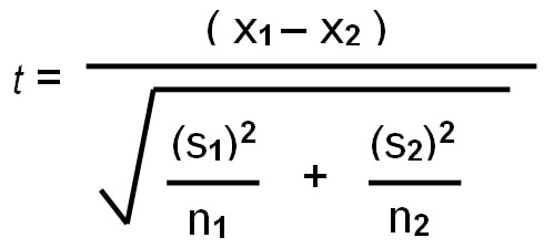
x1 and x2 our the means for the two groups we are comparing. In this case, we’ll call everyhing with a 1 the treatment group, and 2 the control group.
## [1] 0.02908512s1 and s2 are the standard deviations for the treatment and control group.
And n1 and n2 are the number of observations or the sample size of both groups.
That wasn’t so bad. Then we just throw it all together!
## [1] 1.354094That matches. What was all of that we just did? Essentially, we look at how far the distance between the means is, relative to the variance in the data of both.
One way to intuatively undestand what all that means is to think about what would make the test statistic larger or smaller. A larger difference in means, would produce a larger statistic. Less variance, meaning data that was more tightly clustered, would produce a larger t statistic. And a larger sample size would produce a larger t statistic. Once more, a larger difference, less variation in the data, and more data all make us more certain that differnces are real.
df stands for degrees of freedom, which is the number of independent data values in our sample.
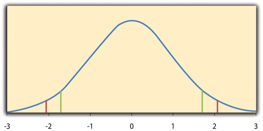
Finally, we have the alternative hypothesis. Here it says “two.sided”. That means we were testing whether the commericals either increased the share of voting, or decreased it - we were looking at both ends or two sides of the distribution. We can specify whether we want to only look at the area above the mean, below the mean, or at both ends as we have done.
Assuming we’re seeking a difference in the means that would only be predicted by chance with a probability of .05, which test is tougher? A two-tailed test. For a two tailed test we seek a p value of .05 at both tails, splitting it with .025 above the mean and .025 below the mean. A one-tailed test places all .05 above or below the mean. Below, the green lines show the cut off at both ends if we only look for the difference in one tail, whereas the red line shows what happens when we look in both tails. This is all to explain why the default option is two.sided, and to generally tell you to let the default stand.
That, was a lot. It might help to walk through another example a bit quicker where we just lay out the basics of a t-test. We can use some polling data for the 1992 election, that asked people who they voted for along with a few demographic questions.
##      vote dem rep female persfinance natlecon clintondis bushdis perotdis
## 1    Bush   0   1      1           1        0     4.0804  0.1024   0.2601
## 2    Bush   0   1      1           0       -1     4.0804  0.1024   0.2601
## 3 Clinton   1   0      1           0       -1     1.0404  1.7424   0.2401
## 4    Bush   0   1      0           0       -1     0.0004  5.3824   2.2201
## 5 Clinton   0   0      1           0       -1     0.9604 11.0220   6.2001
## 6 Clinton   1   0      1          -1       -1     3.9204 18.6620  12.1800
The vote varaible shows who they voters voted for. dem and rep indicate the registered party of voters and females records their gender. The questions persfinance and natlecon indicate whether the respondont thought their personl finances had improved over the previous 4 years (Bush’s first term) and whether the national economy was improving. The other three varaibles require more math than we need right now, but they generally record how distant the voters views are from the candidates.
Let’s see whether personal finances drove people to vote for Bush’s relection.
H0: Personal finance made no difference in the election H1: Voters that felt their personal fiances improved voted more for George Bush
the vote variable has three levels.
##
##   Perot Clinton    Bush
##     183     416     310
We need to create a new variable that indicates just whether people voted for or against Bush, because for a T-test to operate we need two groups. Earlier our two groups were the treatment and the control for whether people watched the tv commercials. Here the two groups are wether people voted for Bush or not.
Rather than splitting the vote92 data set into two halves using subset (like we did earlier) we can just use the ~ operator. ~ is a t1lde mark. ~ can be used to define indicate the varaible being tested (persfinance) and the two groups for our analysis (Bush). This is a little quicker than using subset, and we’ll use the tilde mark in future work in the course.
##
##  Welch Two Sample t-test
##
## data:  persfinance by Bush
## t = -5.6905, df = 662.15, p-value = 1.903e-08
## alternative hypothesis: true difference in means is not equal to 0
## 95 percent confidence interval:
##  -0.4218584 -0.2054129
## sample estimates:
## mean in group 0 mean in group 1
##      -0.1168614       0.1967742
The answer is yes, those who viewed their personal finances as improving were more likely to vote for Bush. The pvalue indicates that the difference in means between the two groups was highly unlikely to have occured by chance. It is not impossible, but it is highly unlikely so we can declare there is a significant difference.
9.4 Populations and samples
Let’s think more about the example we just did. With the the 1992 eletion data, we declared that people with improving personal finances were more likely to vote for Bush. Why do we need test anything about them, we know who they voted for? It’s beause we have a sample of respondents, similar to an exit poll, but what we’re concnered about is all voters. We want to know if people outside the 909 we have data for were more likly to vote for Bush if their personal finances improved. That’s what the test is telling us, that there is a difference in the population (all voters). Just looking at the means between the two groups tells us that there is a difference in our sample. But we rarely care about the sample, what concerns us is projecting or inferring the qualities of others we haven’t asked.
9.5 The problem with .05
That brings us to discuss the .05 test more directly. What would it have meant if the P value had been .06. Well, we would have failed to reject the null. We wouldn’t feel confident enough to say there is a difference in the population. But there would still be a difference in the sample.
Is there a large difference between a P value of .04 and .05 and .06? No, not really. and .05 is a fairly arbitrary standard. Probabilities exist as a continuoum without clear cut offs. A P value of .05 means we’re much more confident than a P value of .6 and a little more confident than a P value of .15. The standard for such a test has to be set somewhere, but we shouldn’t hold .05 as a golden standard.
What does a probability of .05 mean? Let’s think back to the chapter on probability’ it’s equivalent to 1/20. When we set .05 as a standard for hypothesis testing, we’re saying we want to know that there is only a 1 in 20 chance that the difference in voting rates created by the Rock The Vote commercials is by random luck, and to know that 19 out of 20 times it’ll be a true difference between the groups.
So when we get a P value of .05 and reject the null hypothesis, we’re doing so because we think a difference between the two groups is most likely explained by the commercials (or whatever we’re testing). But implicit in a .05 P value is that random chance isn’t impossible, just unlikely. But there is still a 1/20 chance that the difference in voting rates seen after the commercials just occured by random chance and had nothing to do with the commercial. And similarly to flipping a coin, if we do 20 seperate tests in one of them we’ll get a significant value that is generated by random chance. That is a false positive, and we can never identify it.
One approach then is to set a higher standard. We could only reject a null hypothesis if we get a P value of .01 or lower. That would mean only 1 in 100 significant results would be from chance along. Or we could use a standard of .001. That would help to reduce false positives, but not eliminate them still.
.05 has been described as the standard for rejecting the null hypothesis here, but it’s really more of a minimum. Scholars prefer their P values to be .01 or lower when possible, but generally accept .05 as indicative of a significant difference.
9.6 One more problem
Let’s go back to how we calculated P values.
How can we get a larger t-statistic and be more likely to get a significant result? Having a larger difference in the means is one way. That would mean the numerator would get larger. The other way is to make the denomenator smaller, so that whatever the difference in the means is comparatively larger.
If we grow the size of our sample, the n1 and n2, that would shrink the denomenator. That makes intuative sense too. We shouldn’t be very confident if we talk to 10 people and find out that the democrats in the group like cookies more than the republicans. But if we talked to 10 million people, that would be a lot of evidence to disregard if there was a difference in our mean. As we grow our sample size, it becomes more likely that any difference in our means will create a significant finding with a P value of .05 or smaller.
That’s good right? It means we get more precise results, but it creates another concern. When we use larger quantitives of data it becomes necessary to ask whether the differences are significant, as well as large. If I surveyed 10 million voters and found that 72.1 percent of democrats like cookies and only 72.05 republicans like cookies, would the difference be significant?
##
##  Welch Two Sample t-test
##
## data:  dem and rep
## t = 808.95, df = 1e+07, p-value < 2.2e-16
## alternative hypothesis: true difference in means is not equal to 0
## 95 percent confidence interval:
##  2.042372 2.052293
## sample estimates:
## mean of x mean of y
##  72.09836  70.05102
Yes, that finding is very very significant. Is it meaningful? Not really. There is a statistical difference between the two groups, but that difference is so small it doesn’t help someone to plan a party or pick out deserts. With large enough samples the color of your shirt might impact pay by .13 cents or putting your left shoe on first might add 79 minutes to your life. But those differences lack magnitude to be valuable. Thus, as data sets grow in size it becomes important to test for significance, but also the magnitude of the differences to find what’s meaningfull. Unfortunately, evaluating whether a difference is large is a matter of opinion, and can’t be tested for with certainty.
Those are the basics of hypothesis tests with t-tests. We’ll continue to expand on the tests we can run in the following chapters. Next we’ll talk about a specific instance where we use the tools we’ve discussed: polling.